Statistische Modellen voor Communicatieonderzoek (77522101AY)
Resume
SMCR Summary of 'A Gentle but Critical Introduction to Statistical Inference, Moderation, and Mediation'
59 vues 2 fois vendu
Cours
Statistische Modellen voor Communicatieonderzoek (77522101AY)
Établissement
Universiteit Van Amsterdam (UvA)
This document contains the summarized notes (Chapters 1-11) of 'A Gentle but Critical Introduction to Statistical Inference, Moderation, and Mediation' by Wouter de Nooy. All info is organized into headers and subheaders. It includes what assumptions you need to meet for different statistical test...
Sampling distribution
- Requires random samples
- Requires an unbiased estimator
- Continuous versus discrete: probability density versus probabilities.
- Impractical: fuckload of samples needed to create a ‘representative’ distribution e.g. time n effort
Sampling statistic: a number describing a characteristic of a sample. (random variable)
Sampling space: All possible sample statistic values
Sampling distribution: all possible sample statistic values and their probabilities or probability densities.
Probably density: a means of getting the probability that a continuous random variable ( like a sample
statistic) falls within a particular range.
Random variable: a variable with values that depend on chance.
Expected value/expectation: the mean of probability distribution, such as sampling distribution.
Unbiased estimator: a sample statistic for which the expected value equals the population value.
The sampling distribution tells us all possible samples that we could have drawn. Probability of buying a
bag with 5 yellow candies : number of samples with 5 yellow candies / total number of samples drawn
Changing absolute frequencies in the sampling distribution to proportions (relative frequencies) gives
the probability distribution of the sample statistic: A sampling space with a probability (0-1) for each
outcome of the sample statistic.
Discrete value: only limited numbers of outcomes are possible (for this, we use probabilities)
Probabilities
- Proportion: number between 0-1
, - Percentage: between 0%-100%
Mean of sampling distribution (expected value) = population statistic (parameter) → unbiased
estimator.
A sample statistic is an unbiased estimator of the population statistic if the expected value (mean of
sampling distribution) is equal to the population statistic (parameter)
A sample is representative of a population if variables in the sample are distributed in the same way as in
the population. Due to chance, this is unlikely, but we say it is in principle representative and then use
probability theory to account for misrepresentation in the actual drawn sample → confidence intervals
and 0-hypothesesOf course, we know that a random sample is likely to differ from the population due to
chance, so the actual sample that we have drawn is usually not representative of the population.
With continuous sample statistics, drawing a specific average sample statistics is unlikely and thus
nonsensical. We solve this by looking at a range of values instead of a single value. Then how can we
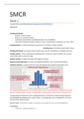
display probabilities? We have to display a probability as an area between the horizontal axis and a curve.
This curve is called a probability density function, so if there is a label to the vertical axis of a continuous
probability distribution, it usually is “Probability density” instead of “Probability”.
A probability density function can give us the probability of values between two thresholds.
Left-hand probability: the probability of
values up to (and including) a threshold
value
Right-hand probability: probably of values
above (and including) a threshold value.
In a null hypothesis significance test, right-
hand and left-hand probabilities are used to
calculate p values.
This is a right-hand probability because it specifies a threshold value (2.8) and all values that are larger. It
concerns the right-hand tail of the sampling distribution.
,Week 2
Chapter 2
Three ways of constructing a sampling distribution with only one sample
1. Bootstrapping: taking one sample and letting the computer generate thousands of samples from
that one sample to create a sampling distribution.
a. Limitation: bootstrapping only works when the one sample we took is more or less
representative of the population (must be randomly sampled and preferably from a big
population). The bootstrap samples must be exactly same size as og sample.
b. However, we can use bootstrapping for any sample statistic. It is more or less the only
way to get a sampling distribution for the sample median
2. The exact approach: calculating the true sampling distribution as the probabilities of
combinations of values on categorical variables
a. Limitation: We can only list all combination if the original variable is categorical/discrete
(e.g. yellow or not yellow). Continuous variables yield an infinite number of possibilities.
b. Limitation: Computer intensive
c. However: it creates a true sampling distribution
3. Theoretical approximation: using a theoretical probability distribution as an approximation of
the sampling distribution
a. Limitation: always approximation, not the true sampling distribution. If requirements
(like sample size) are not met, this approximation can be far-fetched.
Bootstrapping must be done with replacement: if we bootstrap without we will always get exact copies of
the original sample.
Calculating with replacement makes calculations easier, because proportions always stay the same. When
u want to know the percentage of yellow candies and you sample 2, the percentage of yellow candies
stays the same. If you don’t use replacement the percentage decreases slightly.
In an empirical research project, then, we always sample respondents (and so on) without replacement
but our statistical software calculates probabilities as if we sampled with replacement.
Independent samples: samples that can in principle be drawn separately
Dependent/paired samples: the composition of a sample depends partly or entirely on the composition
of another sample (like sample of children and sample of children’s aprents)
*Bootstrapping in SPSS:
- Recommended number of samples is 5000
- Check the ‘seed for Marianna Twister’ if you want the bootstrap sampling to be the same (seeing
as you randomly sample when bootstrapping, it would yield different results every time)
- For confidence interval, check ‘bias corrected accelerated’
*Exact approach
- Usually non-parametric test for categorical variables (nonparametric tests > legacy dialogs >
select)
- However, we will likely calculate for cross tabs (descriptive stat >crosstabs)
o In addition to ‘exact’ option, we need to select a statistics test (e.g. chi-square + Phi and
Cramers V)
, o In ‘cells’, select columns for percentages
o In output, check Fisher’s exact test (its P-value) and (in this example), Cramer’s V/
- Select ‘Exact’ option
- You can set time limit for test
- When executing a cross tabs, also specify which test you will execute (chi-square, etc.) etc.
*Theoretical approximation
- Check if conditions are met: spss does the rest
- Theoretical distributions fit sampling distributions betters if the sample is larger.
- The rule of thumb for using the normal distribution as the sampling distribution of a sample
proportion combines the two aspects by multiplying them and requiring the resulting product to
be larger than five. If the probability of drawing a yellow candy is .2 and our sample size is 30,
the product is .2 * 30 = 6, which is larger than five. That’s good.
o This rule of thumb uses one minus the probability if the probability is larger than .5.
- There are other theoretical distributions beside the normal distribution.
o Binomial distribution for a proportion
o t distribution for 1/2 sample means, regression coefficients and correlation coefficients,
o the F distribution for comparison of variances and comparing means for three or more
groups (analysis of variance, ANOVA),
o the chi-squared distribution for frequency tables and contingency tables.
To check strength of association, the correct measure of association should be selected:
**However, when one checks for a
Nominal Ordinal third variable in 2x2 (whether
Symmetric Cramer’s V* or Phi** Gamma spurious, moderation etc.) one
Assymetric Goodman & Kruskal tau (Lambda) Somer’s d should check the Chi-square.
* = 0-1 scale, others -1-+1 However, when checking the effect
**= Phi for 2x2 tabs, Cramer’s V else. size, one should check Phi.
Nominal/ordinal → check for the lowest one. If one is nominal and other ordinal, go with nominal.
Les avantages d'acheter des résumés chez Stuvia:
Qualité garantie par les avis des clients
Les clients de Stuvia ont évalués plus de 700 000 résumés. C'est comme ça que vous savez que vous achetez les meilleurs documents.
L’achat facile et rapide
Vous pouvez payer rapidement avec iDeal, carte de crédit ou Stuvia-crédit pour les résumés. Il n'y a pas d'adhésion nécessaire.
Focus sur l’essentiel
Vos camarades écrivent eux-mêmes les notes d’étude, c’est pourquoi les documents sont toujours fiables et à jour. Cela garantit que vous arrivez rapidement au coeur du matériel.
Foire aux questions
Qu'est-ce que j'obtiens en achetant ce document ?
Vous obtenez un PDF, disponible immédiatement après votre achat. Le document acheté est accessible à tout moment, n'importe où et indéfiniment via votre profil.
Garantie de remboursement : comment ça marche ?
Notre garantie de satisfaction garantit que vous trouverez toujours un document d'étude qui vous convient. Vous remplissez un formulaire et notre équipe du service client s'occupe du reste.
Auprès de qui est-ce que j'achète ce résumé ?
Stuvia est une place de marché. Alors, vous n'achetez donc pas ce document chez nous, mais auprès du vendeur thaomynguyen. Stuvia facilite les paiements au vendeur.
Est-ce que j'aurai un abonnement?
Non, vous n'achetez ce résumé que pour €7,99. Vous n'êtes lié à rien après votre achat.