KARPAGAM ACADEMY OF HIGHER EDUCATION, COIMBATORE
Class: I MBA Course Name: Managerial Economics
Course Code: 21MBAP103 Unit II Semester: I Year: 2021 -23 Batch
UNIT-II –Production and Cost Function
SYLLABUS
Unit – II : Producer’s Behaviour and Supply : Basic Concepts in Production – Firm – Fixed &
Variable Factors – Short & Long run – Total product – Marginal Product – Average Product –
Production Function – Short-run production function – Long-run production function - Economies and
Diseconomies of Scale – Producer’s Equilibrium. Cost and Revenue Function : Cost of production –
Types of costs - Opportunity Cost – Fixed and Variable costs – Total Cost Curves – Average Cost
Curves – Marginal Cost – Long run and Short run Cost Curves – Total Revenue – Average Revenue –
Marginal Revenue – Break Even Point Analysis.
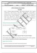
Meaning of Production and Production Function
The concept of production can be represented in the following manner.
The term “Production” means transformation of physical “Inputs” into physical “Outputs”.
The term “Inputs” refers to all those things or items which are required by the firm to produce a particular
product. Four factors of production are land, labor, capital and organization.
PRODUCTION FUNCTION
The entire theory of production centre round the concept of production function.
Prepared by C.Sagunthala, Assistant Professor, Dept of Management, KAHE, Page 1/45
, KARPAGAM ACADEMY OF HIGHER EDUCATION, COIMBATORE
Class: I MBA Course Name: Managerial Economics
Course Code: 21MBAP103 Unit II Semester: I Year: 2021 -23 Batch
“A production Function” expresses the technological or engineering relationship between physical
quantity of inputs employed and physical quantity of outputs obtained by a firm”.
It specifies a flow of output resulting from a flow of inputs during a specified period of time. A production
function can be represented in the form of a mathematical model or equation as Q = f (L, N, K….etc) where
Q stands for quantity of output per unit of time and L N K etc are the various factor inputs like land, capital
labor etc which are used in the production of output. The rate of output Q is thus, a function of the factor
inputs L N K etc, employed by the firm per unit of time.
Factor inputs are of two types.
1. Fixed Inputs. Fixed inputs are those factors the quantity of which remains constant irrespective of
the level of output produced by a firm. For example, land, buildings, machines, tools, equipments,
superior types of labor, top management etc.
2. Variable inputs. Variable inputs are those factors the quantity of which varies with variations in
the levels of output produced by a firm For example, raw materials, power, fuel, water, transport and
communication etc.
The distinction between the two will hold good only in the short run. In the long run, all factor inputs will
become variable in nature.
Short run is a period of time in which only the variable factors can be varied while fixed factors like
plants, machineries, top management etc would remain constant.
Time available at the disposal of a producer to make changes in the quantum of factor inputs is very much
limited in the short run.
Long run is a period of time where in the producer will have adequate time to make any sort of
changes in the factor combinations.
Generally speaking, there are two types of production functions. They are as follows.
Prepared by C.Sagunthala, Assistant Professor, Dept of Management, KAHE, Page 2/45
, KARPAGAM ACADEMY OF HIGHER EDUCATION, COIMBATORE
Class: I MBA Course Name: Managerial Economics
Course Code: 21MBAP103 Unit II Semester: I Year: 2021 -23 Batch
1. Short Run Production Function
In this case, the producer will keep all fixed factors as constant and change only a few variable factor inputs.
In the short run, we come across two kinds of production functions-
1. Quantities of all inputs both fixed and variable will be kept constant and only one variable input will be
varied. For example, Law of Variable Proportions.
2. Quantities of all factor inputs are kept constant and only two variable factor inputs are varied. For
example, Iso-Quants and Iso- Cost curves.
2. Long Run Production Function
In this case, the producer will vary the quantities of all factor inputs, both fixed as well as variable in the
same proportion. For Example, The laws of returns to scale.
Each firm has its own production function which is determined by the state of technology, managerial
ability, organizational skills etc of a firm. If there are any improvements in them, the old production
function is disturbed and a new one takes its place. It may be in the following manner:-
The quantity of inputs may be reduced while the quantity of output may remain same.
The quantity of output may increase while the quantity of inputs may remain same.
The quantity of output may increase and quantity of inputs may decrease.
LAWS OF DIMINISHING RETURNS
The concept of returns to scale is a long run phenomenon. In this case, we study the change in output when
all factor inputs are changed or made available in required quantity. An increase in scale means that all
factor inputs are increased in the same proportion. In returns to scale, all the necessary factor inputs are
increased or decreased to the same extent so that whatever the scale of production, the proportion among the
factors remains the same.
Prepared by C.Sagunthala, Assistant Professor, Dept of Management, KAHE, Page 3/45
, KARPAGAM ACADEMY OF HIGHER EDUCATION, COIMBATORE
Class: I MBA Course Name: Managerial Economics
Course Code: 21MBAP103 Unit II Semester: I Year: 2021 -23 Batch
Three Phases of Returns to Scale
When the quantity of all factor inputs are increased in a given proportion and output increases more than
proportionately, then the returns to scale are said to be increasing; when the output increases in the same
proportion, then the returns to scale are said to be constant; when the output increases less than
proportionately, then the returns to scale are said to be diminishing.
Total Product
S. NS.NO Scale Marginal Product in units
in Units
1 1 Acre of land + 3 labor 5 5
2 2 Acre of land + 5 labor 12 7
3 3 Acre of land + 7 labor 21 9
4 4 Acre of land + 9 labor 32 11
5 5 Acre of land + 11 labor 43 11
6 6 Acre of land + 13labor 54 11
7 7 Acre of land + 15 labor 63 9
8 8 Acre of land + 17 labor 70 7
It is clear from the table that the quantity of land and labor (Scale) is increasing in the same proportion, i.e.
by 1 acre of land and 2 units of labor through out in our example. The output increases more than
proportionately when the producer is employing 4 acres of land and 9 units of labor. Output increases in the
same proportion when the quantity of land is 5 acres and 11units of labor and 6 acres of land and 13 units of
labor. In the later stages, when he employs 7 & 8 acres of land and 15 & 17 units of labor, output increases
less than proportionately. Thus, one can clearly understand the operation of the three phases of the laws of
returns to scale with the help of the table.
Diagrammatic representation
In the diagram, it is clear that the marginal returns curve slope upwards from A to B, indicating increasing
returns to scale. The curve is horizontal from B to C indicating constant returns to scale and from C to D,
the curve slope downwards from left to right indicating the operation of diminishing returns to scale.
Prepared by C.Sagunthala, Assistant Professor, Dept of Management, KAHE, Page 4/45
The benefits of buying summaries with Stuvia:
Guaranteed quality through customer reviews
Stuvia customers have reviewed more than 700,000 summaries. This how you know that you are buying the best documents.
Quick and easy check-out
You can quickly pay through credit card or Stuvia-credit for the summaries. There is no membership needed.
Focus on what matters
Your fellow students write the study notes themselves, which is why the documents are always reliable and up-to-date. This ensures you quickly get to the core!
Frequently asked questions
What do I get when I buy this document?
You get a PDF, available immediately after your purchase. The purchased document is accessible anytime, anywhere and indefinitely through your profile.
Satisfaction guarantee: how does it work?
Our satisfaction guarantee ensures that you always find a study document that suits you well. You fill out a form, and our customer service team takes care of the rest.
Who am I buying these notes from?
Stuvia is a marketplace, so you are not buying this document from us, but from seller Raja05. Stuvia facilitates payment to the seller.
Will I be stuck with a subscription?
No, you only buy these notes for $10.49. You're not tied to anything after your purchase.