CHAPTER 1
Introduction
1.1
1.
For � > 3∕2, the slopes are negative, therefore the solutions are decreasing. For � < 3∕2, the
slopes are positive, hence the solutions are increasing. The equilibrium solution appears to be
�(�) = 3∕2, to which all other solutions converge.
2.
For � > 3∕2, the slopes are positive, therefore the solutions increase. For � < 3∕2, the slopes
are negative, therefore, the solutions decrease. As a result, � diverges from 3∕2 as � → ∞ if
�(0) 3∕2.
3.
For � > −1∕2, the slopes are negative, therefore the solutions decrease. For � < −1∕2, the
slopes are positive, therefore, the solutions increase. As a result, � → −1∕2 as � → ∞.
1
,2 CHAPTER 1 Introduction
4.
For � > −1∕2, the slopes are positive, and hence the solutions increase. For � < −1∕2, the
slopes are negative, and hence the solutions decrease. All solutions diverge away from the
equilibrium solution �(�) = −1∕2.
5. For all solutions to approach the equilibrium solution �(�) = 2∕3, we must have � ′ < 0 for
� > 2∕3, and � ′ > 0 for � < 2∕3. The required rates are satisfied by the differential equation
� ′ = 2 − 3�.
6. For solutions other than �(�) = 2 to diverge from � = 2, �(�) must be an increasing func-
tion for � > 2, and a decreasing function for � < 2. The simplest differential equation whose
solutions satisfy these criteria is � ′ = � − 2.
7.
For � = 0 and � = 4 we have � ′ = 0 and thus � = 0 and � = 4 are equilibrium solutions. For
� > 4, � ′ < 0 so if �(0) > 4 the solution approaches � = 4 from above. If 0 < �(0) < 4, then
� ′ > 0 and the solutions “grow” to � = 4 as � → ∞. For �(0) < 0 we see that � ′ < 0 and the
solutions diverge from 0.
8.
Note that � ′ = 0 for � = 0 and � = 5. The two equilibrium solutions are �(�) = 0 and �(�) = 5.
Based on the direction field, � ′ > 0 for � > 5; thus solutions with initial values greater than
5 diverge from the solution �(�) = 5. For 0 < � < 5, the slopes are negative, and hence solu-
tions with initial values between 0 and 5 all decrease toward the solution �(�) = 0. For
� < 0, the slopes are all positive; thus solutions with initial values less than 0 approach the
solution �(�) = 0.
, 1.1 3
9.
Since � ′ = � 2 , � = 0 is the only equilibrium solution and � ′ > 0 for all �. Thus � → 0 if the
initial value is negative; � diverges from 0 if the initial value is positive.
10.
Observe that � ′ = 0 for � = 0 and � = 2. The two equilibrium solutions are �(�) = 0 and
�(�) = 2. Based on the direction field, � ′ > 0 for � > 2; thus solutions with initial values
greater than 2 diverge from �(�) = 2. For 0 < � < 2, the slopes are also positive, and hence
solutions with initial values between 0 and 2 all increase toward the solution �(�) = 2. For
� < 0, the slopes are all negative; thus solutions with initial values less than 0 diverge from the
solution �(�) = 0.
11. -(�) � ′ = 2 − �.
12. From Figure 1.1.6 we can see that � = 2 is an equilibrium solution and thus (c) and (j) are
the only possible differential equations to consider. Since ��∕�� > 0 for � > 2, and ��∕�� < 0
for � < 2 we conclude that (c) is the correct answer: � ′ = � − 2.
13. -(�) � ′ = −2 − �.
14. -(�) � ′ = 2 + �.
15. From Figure 1.1.9 we can see that � = 0 and � = 3 are equilibrium solutions, so (e) and
(h) are the only possible differential equations. Furthermore, we have ��∕�� < 0 for � > 3 and
for � < 0, and ��∕�� > 0 for 0 < � < 3. This tells us that (h) is the desired differential equation:
� ′ = � (3 − �).
16. -(�) � ′ = � (� − 3).
17. (a) Let �(�) denote the amount of chemical in the pond at time �. The amount � will be
measured in grams and the time � will be measured in hours. The rate at which the chemical
is entering the pond is given by 300 gal/h ⋅ .01 g/gal = 3 g/h. The rate at which the chemical
leaves the pond is given by 300 gal/h ⋅ �∕106 g/gal = (3 × 10⁻⁴ )� g/h. Thus the differential
equation is given by ��∕�� = 3 − (3 × 10⁻⁴ )�.
(b) The equilibrium solution occurs when �′ = 0, or � = 104 grams. Since �′ > 0 for � < 104
g and �′ < 0 for � > 104 g, all solutions approach the equilibrium solution independent of the
amount present at � = 0.
(c) Let �(�) denote the amount of chemical in the pond at time �. From part (a) the
function �(�) satisfies the differential equation ��∕�� = 3 − (3 × 10⁻⁴ )�. Thus in terms of
the concentration �(�) = �(�)∕106 , ��∕�� = (1∕106 )(��∕��) = (1∕106 )(3 − (3 × 10⁻⁴ )�) = (3 ×
10−6 ) − (10−6 )(3 × 10⁻⁴ )� = (3 × 10⁻⁶ ) − (3 × 10⁻⁴ )�.
, 4 CHAPTER 1 Introduction
18. The surface area of a spherical raindrop of radius � is given by � = 4��2 . The volume of a
spherical raindrop is given by � = 4��3 ∕3. Therefore, we see that the surface area � = �� 2∕3
for some constant �. If the raindrop evaporates at a rate proportional to its surface area, then
��∕�� = −�� 2∕3 for some � > 0.
19. The difference between the temperature of the object and the ambient temperature
is � − 70 (� in ◦ F). Since the object is cooling when � > 70, and the rate constant is
� = 0.05 min−1 , the governing differential equation for the temperature of the object is
��∕�� = −.05 (� − 70).
20. (a) Let �(�) be the total amount of the drug (in milligrams) in the patient’s body at any
given time � (hr). The drug enters the body at a constant rate of 500 mg/hr. The rate at which
the drug leaves the bloodstream is given by 0.4 �(�). Hence the accumulation rate of the drug
is described by the differential equation ��∕�� = 500 − 0.4 � (mg/hr).
(b)
Based on the direction field, the amount of drug in the bloodstream approaches the equilib-
rium level of 1250 mg (within a few hours).
21. (a) Following the discussion in the text, the differential equation is �(��∕��) =
�� − � � 2 , or equivalently, ��∕�� = � − �� 2 ∕�.
√ a long time, ��∕�� ≈ 0. Hence the object attains a terminal velocity given by
(b) After
�∞ = ��∕� .
2
(c) Using the relation � �∞ = ��, the required drag coefficient is � = 2∕49 kg/s.
(d)
22.
All solutions become asymptotic to the line � = � − 3 as � → ∞.