Even though this summary was written at the start of my bachelor, the content is still the same and is all condenced into this 30 page summary. The summary is based off ALL video lectures, slides, and readings from the book: "Macroeconomics" by N G. Mankiw. The summary also includes handmade graphs...
Models = simplified theories that show the key relationships among economic variables. The
exogenous variables are those that come from outside the model, they go into the model, what
comes out/what we are able to investigate using the model are the endogenous variables.
GDP measures the value of currently produced goods, if a company makes cars but doesn't sell
them yet, this is seen as an investment. Hence, if a company produces cars in one year, but
sells them the next, then GDP in the first year is affected, but not in the second (since I goes
down when NX or domestic c goes up in the second).
Intermediate goods & value added, just add the different ADDED values until the good is made;
that’s your good value, hence how much affects GDP. If it buys something for 25k, adds 10k
value, then 10k is what affects GDP.
Nominal GDP; value of goods and services measured at current prices. (inflation thus affects
nominal but not real GDP).
Real GDP; value of goods and services measured using constant prices (base prices).
𝑁𝑜𝑚𝑖𝑛𝑎𝑙 𝐺𝐷𝑃
GDP deflator; 𝑅𝑒𝑎𝑙 𝐺𝐷𝑃
→ reflects what is happening to the overall level of prices in the
economy.
GDP = C + I + G + NX (X-I)
GNP = GDP + Factor payments from abroad - factor payments to abroad (looks at total income
earned by nationals).
NNP (net national income) = GNP - depreciation
CPI = takes current price of basket (so using current prices) and divides it by the value of the
basket using the base year prices. CPI only measures the basket goods, while GDP deflator
measures all of the goods. GDP deflator includes only the goods produced domestically, the CPI
doesn’t. Lastly, the CPI assigns fixed weights to the prices of different goods while the GDP
deflator assigns changings weights. CPI also tends to overstate inflation, it also does not take
into account new goods that people might be consuming and it doesn't take into account the
changing quality of goods.
,Chapter 3
Closed Economy - National Income
Supply Side;
We assume that all production depends on A, K, L → 𝑌 = 𝐴 * 𝐹(𝐾, 𝐿)
We assume that A, K, L are constant, so Y is constant too → 𝑌 = 𝐴 * 𝐹(𝐾, 𝐿), so it does
not depend on C, G, I or NX.
Economy is closed, so GDP = GNI
w = wage rate, r = rental price of K. We assume that firms take w, r & P as given and that
they want to max profits; so this means that firms will hire labor as long as real wage (cost) <
MPL and buy capital as long as real cost of capital < MPK. Hence;
𝑤 𝑟
𝑃
= 𝑀𝑃𝐿 -- 𝑃
= 𝑀𝑃𝐾
Total real labor income; 𝑀𝑃𝐿 * 𝐿 -- Total real capital income; 𝑀𝑃𝐾 * 𝐾 → since economy is
closed and we have constant returns to scale, 𝑌 = 𝑀𝑃𝐿 * 𝐿 + 𝑀𝑃𝐾 * 𝐾
Conclusion; Production is chosen by K & L and it is constant bcz of this. We have constant
returns to scale (assumption), so GDP is fully distributed between K & L, no excess profits.
Quick approximations of changes in K or L on Y;
If x*y; then we do gx + gy (change x + change y) → approx change.
If x/y then we do gx - gy (change x - change y) → approx change.
If x^a then we do a*gx (change x * a) → approx change.
For a cobb-douglas production function, labor/capital share is the exponent of labor/capital
α 1−α
times Y → for 𝑌 = 𝐴 * 𝐾 𝐿 → 𝐿 𝑠ℎ𝑎𝑟𝑒 = (1 − α)𝑌; 𝐾 𝑠ℎ𝑎𝑟𝑒 = α𝑌
Demand Side;
- 3 components → C, I, G (no NX bcz we are in a closed economy)
C depends on Y-T (disposable income) so; 𝐶 = 𝐶(𝑌 − 𝑇). The slope is MPC and Y intercept is
the autonomous consumption (consumption that happens even if there is 0 income/disposable
income.
I is a function of r (real interest rate); 𝐼 = 𝐼(𝑟). The relationship between I and r is opposite,
hence an increase in I means a decrease in r. The cost of borrowing money to invest, aka the
cost of investing is thus r.
G is exogenous, so is T. This is an assumption. Transfer payments are not a part of G. Hence,
G and T are both given!!!
, Since demand is 𝐶 + 𝐼 + 𝐺 = 𝐶(𝑌 − 𝑇) + 𝐼(𝑟) + 𝐺 and supply is 𝑌 = 𝐴 * 𝐹(𝐾, 𝐿) = 𝑌we
can see that equilibrium happens at; 𝑌 = 𝐶(𝑌 − 𝑇) + 𝐼(𝑟) + 𝐺 → only I(r) can change so we
know that the real interest rate establishes equilibrium on the market for goods and services.
Price does not play a role!
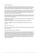
In the financial market → one asset = loanable funds. The demand for loanable funds is
investment (I) and the supply is national savings (in a closed economy). The price of loanable
funds is the real interest rate (r).
Investment (I) is the investment by firms and consumers.
𝑝
Savings S has two parts, private savings (𝑆 = (𝑌 − 𝑇) − 𝐶(𝑌 − 𝑇)) and
𝑔
government savings (𝑆 = 𝑇 − 𝐺) Since S = Sp+Sg we can see that
𝑛
𝑆 = (𝑌 − 𝑇) − 𝐶(𝑌 − 𝑇) + 𝑇 − 𝐺 so; 𝑆 = 𝑆 → constant! Let's take a look at the graph;
- Exogenous variables; A,K,L,G,T
- Endogenous variables; Y, C, S, I, r
- Equations;
- 𝑌 = 𝐴 * 𝐹(𝐾, 𝐿)
- 𝐶 = 𝐶(𝑌 − 𝑇)
- 𝐼 = 𝐼(𝑟)
- 𝑆=𝑌−𝐶−𝐺
- 𝑆=𝐼
- Y is determined by K and L, not C, I or
G!!!
- Equilibrium in 1 market = equilibrium
in the other. All variables are real so
money does not play a role in the long
run!
Last video on chapter 3 (week 2) goes over case studies; good for review, you can guess what
happens using this model.
Conclusions;
- Production is determined by available K and L and A
- Real interest rate adjusts to bring equilibrium in the market for goods and services;
C+I+G = Y.
- Which leads to equilibrium in market for loanable funds S=I
- A change in G or T does not affect Y, but it does affect I or C.
- Nominal variables like P or amount of money do not have a role.
The benefits of buying summaries with Stuvia:
Guaranteed quality through customer reviews
Stuvia customers have reviewed more than 700,000 summaries. This how you know that you are buying the best documents.
Quick and easy check-out
You can quickly pay through credit card or Stuvia-credit for the summaries. There is no membership needed.
Focus on what matters
Your fellow students write the study notes themselves, which is why the documents are always reliable and up-to-date. This ensures you quickly get to the core!
Frequently asked questions
What do I get when I buy this document?
You get a PDF, available immediately after your purchase. The purchased document is accessible anytime, anywhere and indefinitely through your profile.
Satisfaction guarantee: how does it work?
Our satisfaction guarantee ensures that you always find a study document that suits you well. You fill out a form, and our customer service team takes care of the rest.
Who am I buying these notes from?
Stuvia is a marketplace, so you are not buying this document from us, but from seller mathieuvandevel. Stuvia facilitates payment to the seller.
Will I be stuck with a subscription?
No, you only buy these notes for $8.56. You're not tied to anything after your purchase.