LECTURE 1
Powerpoint lecture – Basic principles of mixed model analysis
Mixed model analysis is an extension from linear regression model analysis.
Linear regression: line drawn with where the dots have the least possible distance to the line best
way to describe linear relationship.
- b0 = value of outcome where independent variable is 0 (where x is 0)
- b1 = relationship between independent variable and outcome
When adjusted for a group different intercepts (b0)
Not efficient to add many dummy variables for all categorical variables (for example: adding 49
dummy variables for 50 different areas) (many dummy variables lead to loss of power and efficiency)
solution: mixed model analysis very efficient way to deal with categorical variables with many
groups.
Mixed model analysis: three steps (instead of adding it as confounder)
1. estimate intercepts for all groups
2. normal distribution over the intercepts
3. estimate the variance of the normal distribution
Mixed model analysis: three steps (instead of adding it as effect modification)
1. estimate regression coefficients for all groups
2. normal distribution over regression coefficients
3. estimate variance of normal distribution
Thus, what is mixed model analysis:
- correction for variable is carried out by estimating the variance of intercepts (‘random
intercept’')
- effect modification with variable is carried out by estimating the variance of the slopes (‘random
slopes’)
Multilevel analysis we have two-level structure 1: subject, 2: area (for example)
Powerpoint lecture – Mixed model analysis with continuous outcome
Two level structure example
- 1: person
- 2: neighborhood
Outcome variable = depression (continuous)
What is the relationship between age and depression?
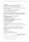
Step 1: Naïve model:
Interpretation: when age differs with
1 unit, depression differs with 0.128
units
,B0 = _cons = value of depression when age=0 (but age is not zero in this situation, thus not
informative)
Step 2: add random intercept on neighborhood level:
var(_cons) variance over the intercept
Log likelihood likelihood ratio test is performed to
evaluate if there is a difference between the models
and therefore if adding random effects is a better
model
likelihood ratio test = difference in -2 log likelihoods
chi-square distributed: number of degrees of
freedom is equal to the difference in number of
parameters between the model in this case: (-2*-954.96) – (-2*-812.60) = 284 (> 3.84)
significant difference second model (most complex) is better!
3.84 (= 1.962) = chi-square distribution with 1 degree of freedom (= critical value higher likelihood
ratio significant difference)
More informative number is measure of dependency
Intraclass correlation coefficient (ICC) = between group variance/total variance
ICC of 0.55 is really high – in real life about 0.10-0.20
the higher the variance between groups the higher the correlation within the group
the lower the variance between groups the lower the correlation within the group
thus correlation and difference are basically the same thing.
Step 3: add random slope for age on neighborhood level
Always model the dependency of
random slope and random
intercept! (cov(age,_cons))
Compare likelihood of unstructured model
with the likelihood of model with only the
random intercept (chi-square distribution
with 2 degrees of freedom 5.99)
here: (-2*-812.60) – (-2*807.25) = 10.7
significant!
- Negative covariance random intercept and random slope lines towards each other
, - Positive covariance random intercept and random slope lines diverge
Random intercept variance has increased (4x) (compared to model without covariance) how is this
possible?
- Random intercept variance reflects the variance on the whole range of age.
- We add a random slope for age to the model + we have a negative covariance
o Negative covariance: higher levels of depression = lower age (and vice versa) (see first
picture above)
o Now the differences between groups (neighborhood) differs along the age range
o The variance along the first part of age range does not say anything (since the real data
starts from around age 40)
o Possible solution: Moving the zero line to the start age? = centering the independent
variable = subtracting the mean value from all observations (you basically move the y-axis to
the minimum age in the sample (040)) better interpretation of intercept and variance.
Does not give a better model (doesn’t influence regression coefficient B1 & log
likelihood is not changed)
What is different? intercept value (we moved the y-axis; makes sense) is now
interpretable
Also different variance over the intercept
Sometimes, when not centering the data, there is no convergence of lines, therefore
no solution therefore
Thus: centering the independent variable makes the intercept and the random variance of the
intercepts better interpretable.
Three level structure example
Basics are the same as in a two level structure.
Levels: person – neighborhood – region
Forward structure:
- Naïve model
- Random intercept on neighborhood level
- Random intercept on region level
o Both random intercepts on neighborhood and region level added different interpretation
now variance around intercept on neighborhood level = difference between
neighborhoods within region
- Random slope for age on neighborhood level
- Random slope for age on region level
Always start with random intercepts (and then slopes).
The benefits of buying summaries with Stuvia:
Guaranteed quality through customer reviews
Stuvia customers have reviewed more than 700,000 summaries. This how you know that you are buying the best documents.
Quick and easy check-out
You can quickly pay through credit card or Stuvia-credit for the summaries. There is no membership needed.
Focus on what matters
Your fellow students write the study notes themselves, which is why the documents are always reliable and up-to-date. This ensures you quickly get to the core!
Frequently asked questions
What do I get when I buy this document?
You get a PDF, available immediately after your purchase. The purchased document is accessible anytime, anywhere and indefinitely through your profile.
Satisfaction guarantee: how does it work?
Our satisfaction guarantee ensures that you always find a study document that suits you well. You fill out a form, and our customer service team takes care of the rest.
Who am I buying these notes from?
Stuvia is a marketplace, so you are not buying this document from us, but from seller Studentje1811. Stuvia facilitates payment to the seller.
Will I be stuck with a subscription?
No, you only buy these notes for $6.15. You're not tied to anything after your purchase.