Hoorcollege 1: Frequentist vs Bayesian statistics and Multiple linear regression
We have 2 di erent approaches with statistics:
1. Frequentist framework: Test how well the data ts the H0 (NHST) Nulhypothese toetsing. We
look at the p-values, con dence intervals, e ect sizes and the power analysis.
2. Bayesian framework: Looks at the probability of the hypothesis given the data, taking prior
information into account. We look at: Bayes factors (BFs), priors, posteriors, credible intervals.
We can try to estimate the value of the parameter (de waarde die een hele populatie beschrijft, bv
populatiegemiddelde). Second we can do: testing hypothesis. We can do this in 2 di erent ways:
1. Frequentist estimation: Empirical research uses collected data to learn from. Information in
this data is captured in a likelihood function ( t of the data). When we move to the right, the
likelihood goes up. All relevant information for inference is contained in the likelihood function.
We don’t have a prior. We ignore this. It is neutral. (Don’t have assumptions).
2. Bayesian estimation: In addition to the data, we may also have prior information about µ.
(E.G the mean in the population). Central idea: prior knowledge is updated with information in
the data and together provides the posterior distribution for µ. The advantage is:
accumulating knowledge (‘today’s posterior is tomorrow’s prior’). Dus het vergaren van kennis.
The disadvantage is that the results depend on the choice of your prior.
We have di erent priors:
1. Uninformed distribution: we have no expectations. It is
complete at. Any value is likely. There is a in nity
2. Bounded uniform: here the in nity makes no sense. We
have boundaries. We do know the range form IQ. Between
this range al values are likely.
3. We still use a range, but we have some prior knowledge
that the IQ is more likely to be in the middle. Values that are
low of high are very onlikely on average. In the middle is it more likely.
4. Peak prior: we have a really strong assumption that average the IQ is in the middle.
5. Informed prior: this is not centered in the middle. We expect the average is quit low. We use
this if we have a speci c group that we want to measure.
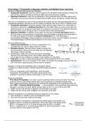
Bayesian vs frequentist probability (blue is bayesian). Bayes
conditions on observed data; whereas frequentist testing conditions
on H0.
- Bayesian: probability of the hypothesis j, given the data.
- Frequentist: The probability of the data, given the H0. How
probable it would be to observe these data, if the H0 is true.
Bayesian probability
- Prior Model Probabilities: how likely is each hypothesis before seeing the data? The most
common choice is that before seeing data, each hypothesis is considered equally likely.
- When testing hypotheses, Bayesians can calculate the probability of the hypothesis given the
data: PMP = Posterior Model Probability —> the probability of the hypothesis after observing
the data. It consists of 2 parts: (Beide kansen tellen op tot 1.0, ook zo bij de prior MP)
1. PMK0: de kans dat H0 waar is gegeven de informatie uit de data
2. PMKa: de kans da Ha waar is gegeven de informatie uit de data
Bayesian probability of a hypothesis being true depends on two criteria:
1. How sensible it is, based on prior knowledge (the prior)
2. How well it ts the new evidence (the data)
Bayesian testing is comparative: hypotheses are tested against one another, not
in isolation. We can compare the hypothesis. This is also seen in the Bayes factor:
- BF10 = 10 Support for H1 is 10 times stronger than for H0 (h1 is better)
- BF10 = 1 Support for H1 is as strong as support for H0 (if we go below 1, then
we know there is more support voor H0)
flfffi ff fi fi fi ff fifi fi ff
, We have a di erent de nition of probability (a di erent probability theory):
- Frequentist: probability is the relative frequency of events (more formal?) In the long run, how
often does something happen. (If we keep repeating it)
- Frequentist 95% con dence interval (CI): If we were to repeat this experiment many times
and calculate a CI each time, 95% of the intervals will include the true parameter value (and
5% won’t). Van de 100 keer dat we een interval berekenen. Hebben we 95 intervallen met de
correcte parameter (gemiddelde waarden die we willen weten) in de interval.
- Bayesian: probability is the degree of belief (more intuitive?) what we believe before (prior
probability) and after (posterior probability) the data.
- Bayesian 95% credible interval: There is 95% probability that the true value is in the
credible interval.
Multiple Linear Regression (MLR)
- A linear regression is with 2 variables, we try to capture the relationship between 2
variables. We try to t a straight line trough the cloud. We get a
Regressievergelijking (regression equation). B0 is the intercept, where the line
starts (snijpunt met de y-as). B1 is the slope; how steep the line is (hoe schijn
loopt de lijn). We use X to predict Y. In reality we add Ei to the formula. This is a
residual (residu). It’s how far the data (dot) lies form the line.
- With a multiple linear regression we use more predictable variables. If we add more predictable
variables, it leads to more spreading (higher R2). And it is a more accurate prediction.
We have model assumptions (voorwaarden). Serious violations lead to incorrect results (the
results doesn’t mean what’s is supposed to mean).
1. MLR assumes interval/ratio variables (outcome and predictors). If there is a categorical
nummer, we need to make it into a dummy variables. MLR can handle dummy variables as
predictors. Each dummy variable is a dichotomous variable that only takes the values 0 and
1. Interpretation of B2: di erence in mean grade between males and females with the same
age. We use the independent variables to predict the dependent variable.
1. Assumption: the dependent (afhankelijke) variable is a continuous measure (interval or
ratio level). Een continue variabelen.
2. Assumption: the independent (onafhankelijke) variables are continuous or dichotomous
(there are two categories).
2. There are linear relationships between the dependent variable and each of the continuous
independent variables. This can be checked using scatterplots. (een rechte lijn)
3. There are no outliers. An outlier is a case that deviates strongly from other cases in the data
set. Outliers can be a problem because they may indicate that a data point is due to an error
and because they can have an outsized impact on the results. Multivariate outliers (for all
variables in the model) can be assessed whilst performing the analysis.
- Standardized residuals: we check whether there are outliers in the Y-space. As a rule of
thumb, it can be assumed that the values must be between -3.3 and +3.3. Those smaller
than -3.3, or greater than +3.3, indicate potential outliers.
- Cook’s Distance: With Cook's distance, it is possible to check whether there are outliers
within the XY-space. An outlier in the XY-space is an extreme combination of X (all X-
variables) and Y scores. It indicates the overall in uence of a respondent on the model. As a
rule of thumb, we maintain that values for Cook’s distance must be lower than 1. Values
higher than 1 indicate in uential respondents (in uential cases).
4. Absence of multicollinearity: Multicollinearity indicates whether the relationship between two
or more independent variables is too strong. Association between predictors is not a problem
for MLR, but very large association (r above .8 / .9) is. If you include overly related variables in
your model, this has three consequences:
- The regression coe cients (B) are unreliable,
- It limits the magnitude of R (the correlation between Y and Ŷ),
- The importance of individual independent variables can hardly be determined, if at all.
- Determining whether multicollinearity is an issue can be done on the basis of the
statistics Tolerance or VIF (Variance In ation Factor). You can use the following rule of thumb:
ff ffifi fifi flff fl ffflfl
The benefits of buying summaries with Stuvia:
Guaranteed quality through customer reviews
Stuvia customers have reviewed more than 700,000 summaries. This how you know that you are buying the best documents.
Quick and easy check-out
You can quickly pay through credit card or Stuvia-credit for the summaries. There is no membership needed.
Focus on what matters
Your fellow students write the study notes themselves, which is why the documents are always reliable and up-to-date. This ensures you quickly get to the core!
Frequently asked questions
What do I get when I buy this document?
You get a PDF, available immediately after your purchase. The purchased document is accessible anytime, anywhere and indefinitely through your profile.
Satisfaction guarantee: how does it work?
Our satisfaction guarantee ensures that you always find a study document that suits you well. You fill out a form, and our customer service team takes care of the rest.
Who am I buying these notes from?
Stuvia is a marketplace, so you are not buying this document from us, but from seller indyborgers. Stuvia facilitates payment to the seller.
Will I be stuck with a subscription?
No, you only buy these notes for $5.63. You're not tied to anything after your purchase.