Test of nominal data (anything we can put into mutually exclusive categories)
People can only fit into one category
When there are 2 options and nobody knows which is right, we might expect 50% of people
choose option A and 50% of people choose option B. However, we must compare the number of
people choosing option A to the number we could expect by chance alone.
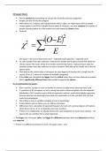
Formula:
Chi square = the sum of (observed count – expected count) squared, / expected count
So, take number from data collection, subtract the number you’d expect to pick that option by
chance, square the result, divide it by number expected by chance, repeat previous steps for
another number from data until you run out of numbers, then add up the results, this is the chi
square value.
Then look up the critical value of chi square for your degrees of freedom (for a single row chi-
square, df are k-1, where k is number of available categories)
If the value you calculated was bigger than the critical value, then you have observed a number
that is significantly different from what would be expected by chance.
R x C (multivariate) chi square:
Row x column; number of rows vs number of columns in table where observed data is put.
A ‘goodness of fit’ chi square, as we’re seeing how well an observed pattern fits the expected
distribution. GoF is another way to think of regression analyses, particularly logistic regression,
because what we are assessing is how close our expectation is to the real data. GoF not that
useful to psychologists.
More likely to have 2 variables changing at once in psychology
If data follows rules as above, you can still use chi square.
Differences here: calculation of expected frequency for each cell, and also degrees of freedom,
which here is (R-1) x (C-1). So basically, just more numbers.
If there is no relationship, we should observe the same proportion of each of our columns – chi
square tells you whether this is what happened.
--> The larger your chi square value, the bigger the difference between what was observed and what
was expected.
--> If there's no difference between O and E, chi square value = zero
,Chi square in Jasp:
No assumptions to be met as it's not possible to have normally distributed data, so therefore all
other assumptions don’t hold
Have to assume independence (belong to one category OR the other, not both)
Also assume there are no expected counts below 5 (chi square value only approximate up until
a certain sample size, where it becomes more accurate)
Frequency menu-->contingency tables, one variable across rows, and the other down the
columns (doesn’t matter which)
Go down cells, click expected counts to check assumption (this relates to sample size and
power)
Click Phi and Cramer’s V. This calculates effect sizes related to Chi square (Phi only shows the
effect size of 2x2 contingency tables, where you have 2 variables each, with 2 levels)
Reporting in APA format: Name of the test, degrees of freedom in parentheses, the value you
calculated for the statistic, the probability value, the effect size.
E.g., "Data was analyzed using chi square which revealed a significant/non-significant (delete as
appropriate) association between [variable x] and [variable y], χ 2 (3) =_ , p = _, [insert effect size
here]."
Short cut to chi square data entry: need to tell Jasp that it should count each row the number of times
that it says in the frequency column. So, by placing ‘frequency’ into the ‘counts’ box, all participants are
now included and there will be a statistically significant value.
Yates’ Continuity Correction:
Chi square can be used in almost the same way in situations where both variables only have 2 levels. Chi
square distribution is biased upwards, so if there’s a smaller amount of data, differences look larger than
they really are (overall swing in data is big)
If we do chi square on a 2x2 contingency table, we use Yates’ correction, to make chi square value
smaller, making it harder to say if there is a significant association between the variables, so we don’t
get it wrong.
Under circumstances where we have small samples and 2x2 contingency tables, the probabilities that
we get from a standard chi square, even with the correction, are not as accurate as we want them. So,
we can use Fisher's exact test (click ‘log odds ratio’). This will be roughly the standard p value, but in
real-world research we might need to use this.
ANCOVA (analysis of covariance)
, Simpler to explain ANCOVA with only one IV
Covariate: another thing we can measure but aren’t interested in – a confound
ANCOVA is a mash up of ANOVA and correlation.
How ANCOVA is calculated:
-Calculate SS as we would in a normal one-way ANOVA, getting a total SS, SS within groups and
SS between groups for the DV.
-Then calculate SS total and SS within groups for the covariate in the same way (but this time
not calculating the between groups version as were not interested in the effect of the IV on the
covariate), then calculate the SS total for our DV & covariate and the shared variance between
the two.
-Then adjust the SS total for the DV to remove the amount of variance that could be attributed
to the covariate.
-Go through same steps with the SS within groups and you get an adjusted set of variance
estimates which are used for an ANOVA, telling you the effect of the IV on the DV without the
covariate getting in the way
Assumptions:
--> Linear relationship between covariate and dependent variable
(Regression-->correlation-->from correlation between the 2 variables-->Pearson's R should be >
0.5 for significance-->if significant, LINEAR)
--> Scores on the covariate should be independent of the IV (shouldn’t be a significant
difference between covariate scores depending on the level of the IV)
(ANOVA--> IV to fixed factors & covariate to DV--> want p value insignificant at > 0.05)
--> Homogeneity of regression slopes (relationship between covariate and DV shouldn’t be
different depending on the level of the IV)
(ANCOVA --> IV to fixed factors, DV to DV & covariate to covariates --> want an insignificant
interaction between the 3; model --> put components together into model terms & this creates
an interaction row in the table --> want p > 0.05
ANCOVA on JASP:
Assumption checks within the ANCOVA:
--> Homogeneity tests gives Levene’s test for equality of variances (amount of variance around
the mean within each level of the IVs should be roughly the same). We want an insignificant p
value, where p > 0.05)
--> QQ plot of residuals gives test of normal distribution of the error term. We want circles to be
close to the line
Want partial eta squared effect size
Run analysis again removing the covariate, then put it back in to make a comparison
Perform post-hoc tests with Bonferroni correction
Turn on descriptive statistics, and look at marginal means – the means after you’ve applied
adjustment, altered to take into account the covariate
Reporting: F (df, error df) = [the value in the F column], p = [the value in the sig column], partial
eta squared = [the value in the partial eta squared column].
The benefits of buying summaries with Stuvia:
Guaranteed quality through customer reviews
Stuvia customers have reviewed more than 700,000 summaries. This how you know that you are buying the best documents.
Quick and easy check-out
You can quickly pay through credit card or Stuvia-credit for the summaries. There is no membership needed.
Focus on what matters
Your fellow students write the study notes themselves, which is why the documents are always reliable and up-to-date. This ensures you quickly get to the core!
Frequently asked questions
What do I get when I buy this document?
You get a PDF, available immediately after your purchase. The purchased document is accessible anytime, anywhere and indefinitely through your profile.
Satisfaction guarantee: how does it work?
Our satisfaction guarantee ensures that you always find a study document that suits you well. You fill out a form, and our customer service team takes care of the rest.
Who am I buying these notes from?
Stuvia is a marketplace, so you are not buying this document from us, but from seller griches10. Stuvia facilitates payment to the seller.
Will I be stuck with a subscription?
No, you only buy these notes for $10.07. You're not tied to anything after your purchase.