100% satisfaction guarantee Immediately available after payment Both online and in PDF No strings attached
logo-home
Solution Manual for Numerical Methods for Engineers 8th edition by Steven C. Chapra, Raymond P. Canale. $17.49   Add to cart

Exam (elaborations)

Solution Manual for Numerical Methods for Engineers 8th edition by Steven C. Chapra, Raymond P. Canale.

2 reviews
 689 views  14 purchases
  • Course
  • SM+TB
  • Institution
  • SM+TB

Solution Manual for Numerical Methods for Engineers 8th edition by Steven C. Chapra, Raymond P. Canale.

Preview 4 out of 1180  pages

  • July 17, 2023
  • 1180
  • 2022/2023
  • Exam (elaborations)
  • Questions & answers
book image

Book Title:

Author(s):

  • Edition:
  • ISBN:
  • Edition:
  • SM+TB
  • SM+TB

2  reviews

review-writer-avatar

By: prem011014 • 7 months ago

review-writer-avatar

By: abdarefa • 10 months ago

avatar-seller
solutions
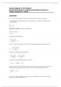
1 Copyright 202 1 © McGraw -Hill Education. All rights reserved. No reproduction or distribution without the prior written consent of McGraw -Hill Education. Solution Manual for All Chapters Numerical Methods for Engineers 8th edition by Steven C. Chapra, Raymond P. Canale CHAPTER 1 1.1 Use calculus to solve Eq. (1.9) for the case where the initial velocity υ(0) is nonzero. We will illustrate two different methods for solving this problem: (1) separation of variables, and (2) Laplace transform. dv cgvdt m Separation of variables : Separation of variables gives 1dv dtcgvm
 The integrals can be evaluated as ln /cgvmtCcm   where C = a constant of integration, which can be evaluated by applying the initial condition to yield ln (0) /cgvmCcm which can be substituted back into the solution ln ln (0) //ccg v g vmmtc m c m            This result can be rearranged algebraically to solve for v,  ( / ) ( / )(0) 1c m t c m t mgv v e ec   where the first part is the general solution and the second part is the particular solution for the constant forcing function due to gravity. For the case where , v(0) = 0, the solution reduces to Eq. (1.10)  ( / )1c m t mgvec 2 Copyright 202 1 © McGraw -Hill Education. All rights reserved. No reproduction or distribution without the prior written consent of McGraw -Hill Education. Laplace transform solution: An alternative solution is provided by applying Laplace transform to the differential equation to give ( ) (0) ( )gcsV s v V ssm   Solve algebraically for the transformed velocity (0)()/ ( / )vgVss c m s s c m (1) The second term on the right of the equal sign can be expanded with partial fractions ( / )
( / ) / ( / )g A B A s c m Bs
s s c m s s c m s s c m     (2) By equating like terms in the numerator, the following must hold 0cg A As Bsm   The first equation can be solved for A = mg/c. According to the second equation, B = –A, so B = –mg/c. Substituting these back into (2) gives //
( / ) /g mg c mg c
s s c m s s c m This can be substituted into Eq. 1 to give (0) / /()//v mg c mg cVss c m s s c m   Taking inverse Laplace transforms yields ( / ) ( / )( ) (0)c m t c m t mg mgv t v e ecc   or collecting terms  ( / ) ( / )( ) (0) 1c m t c m t mgv t v e ec   1.2 Repeat Example 1.2. Compute the velocity to t = 10 s, with a step size of (a) 1 and (b) 0.5 s. Can you mak e any statement regarding the errors of the calculation based on the results? At t = 10 s, the analytical solution is 44.91893 (Example 1.1). The relative error can be calculated with analytical numericalrelative true error 100%analytical The numerical results are: 3 Copyright 202 1 © McGraw -Hill Education. All rights reserved. No reproduction or distribution without the prior written consent of McGraw -Hill Education. step v(10) magnitude of relative error 2 48.0179 6.899 % 1 46.411 2 3.322 % 0.5 45.6509 1.630 % The error versus step size can then be plotted as Thus, halving the step size approximately halves the error. 1.3 Rather than the linear relationship of Eq. (1.7), you might choose to model the upward force on the parachutist as a second -order relationship, UF c v v= - ¢∣∣ where c′ = a bulk second -order drag coefficient (kg/m). Note that the second -order term could be represented as v2 if the parachutist always fell in the downward direction. For the present case, we use the more general representation, vv∣∣ , so that the proper sign is obtained for both the downward and the upward directions. (a) Using calculus, obtain the closed -form solution for the case where the jumper is initially at rest (υ = 0 at t = 0). (b) Repeat the numerical calculation in Example 1.2 with the same initial condition and parameter values, but with second -order drag. Use a value of 0.225 kg/m for cd′. (a) You are given the following differential equation with the initial condition, v(t = 0) = 0, 2 dv cgvdt m Multiply both sides by m/c′ gives 2 m dv mgvc dt c Define / a mg c   0.01.02.03.04.05.06.07.08.0
0 0.5 1 1.5 2 2.5Relative error (%) Step size (seconds) Relative True Error vs. Step size 4 Copyright 202 1 © McGraw -Hill Education. All rights reserved. No reproduction or distribution without the prior written consent of McGraw -Hill Education. 22 m dvavc dt Integrate by separation of variables, 22dv cdtm av
 A table of integrals can be consulted to find that 1
221tanhdx x
aa ax
 Therefore, the integration yields 1 1tanhvctCa a m  If v = 0 at t = 0, then because tanh–1(0) = 0, the constant of integration C = 0 and we obtain the equation 1 1tanhvcta a m  This result can then be rearranged to solve for v tanhgm gcvtcm    (b) Using Euler‘s method, the first two steps are computed 2 0.225(2) 0 9.81 (0) 2 19.6268.1v    2 0.225(4) 19.62 9.81 (1 43 9.62)66.696 4 28.3115 v    The computation can be continued and the results summarized along with the analytical result as: t v-numerical dv/dt v-analytical 0 0 9.81 0 2 19.62 8.538157 18.8138836 4 36.69631454 5.360817 33.61984724 6 47.41794779 2.381162 43.22542283 8 52.18027088 0.814029 48.7004867 10 53.80832813 0.243911 51.59332241 12 54.29615076 0.069674 53.06072073  54.48999908 0 54.48999908

The benefits of buying summaries with Stuvia:

Guaranteed quality through customer reviews

Guaranteed quality through customer reviews

Stuvia customers have reviewed more than 700,000 summaries. This how you know that you are buying the best documents.

Quick and easy check-out

Quick and easy check-out

You can quickly pay through credit card or Stuvia-credit for the summaries. There is no membership needed.

Focus on what matters

Focus on what matters

Your fellow students write the study notes themselves, which is why the documents are always reliable and up-to-date. This ensures you quickly get to the core!

Frequently asked questions

What do I get when I buy this document?

You get a PDF, available immediately after your purchase. The purchased document is accessible anytime, anywhere and indefinitely through your profile.

Satisfaction guarantee: how does it work?

Our satisfaction guarantee ensures that you always find a study document that suits you well. You fill out a form, and our customer service team takes care of the rest.

Who am I buying these notes from?

Stuvia is a marketplace, so you are not buying this document from us, but from seller solutions. Stuvia facilitates payment to the seller.

Will I be stuck with a subscription?

No, you only buy these notes for $17.49. You're not tied to anything after your purchase.

Can Stuvia be trusted?

4.6 stars on Google & Trustpilot (+1000 reviews)

72841 documents were sold in the last 30 days

Founded in 2010, the go-to place to buy study notes for 14 years now

Start selling
$17.49  14x  sold
  • (2)
  Add to cart