Summary Statistics for Business and Economics- BA2, Business Economics
85 views 3 purchases
Course
Statistics For Business And Economics II
Institution
Vrije Universiteit Brussel (VUB)
Book
Business Statistics
This is a summary for the course Statistics for Business and Economics that is given in the second semester of the second semester. This summary is based on the lectures, notes and the book "Business Statistics"
Lecture 2: Sampling distributions and confidence intervals for proportions
1. The distribution of sample proportions: introduction
Population: about who/what do you want to draw conclusion e.g. All residents of Brussels. But we use a Sample if it is not feasible/Very expensive
to survey/study the whole population. If it is possible to use the entire population, we get the population parameter -> proportion p in the
population. If we take a sample, we get the sample statistic -> proportion p̂ in the sample.
Sampling distribution -> To learn more about variability of the sample proportion p̂ , we have to imagine how the sample proportion would vary
across all possible samples.
Sample proportion -> calculated based on only one possible sample taken from the population and variability -> how would the sample
proportion vary across all possible samples?
e.g. if 20% of customers increase their spending on a credit card, the marketing campaign is financially viable, in a sample of 1000 customers, 211
increased their spending, to the campaign is financially viable.
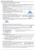
Stimulation of 10 000 sample proportions for a sample size of 1000 with a p = 0.2 not every
sample has a sample proportion equal to 0.2, sample proportion bigger than 0.24 and smaller
than 0.16 are rare, most sample proportions are between 0.18 and 0.22, the histogram shows a
stimulation of the sampling distribution p̂
2. The distribution of sample proportions: sampling distribution
The distribution of proportion over many independent samples from the same population is called the sampling distribution of the proportions.
For distributions that are bell-shaped and centered at the true proportion, p, we can
use the sample size n to find the standard deviation of the sampling distribution:
Difference between sample proportions: sampling error (not really an error, better
called the sampling variability.
Sampling distribution model for the sample proportion won’t work for all situations but it works for most situations
Provided that the sampled values are independent and the sample size is large enough, the sampling distribution of p̂ is modelled by a Normal
model with mean p̂ = p and standard deviation SD(p̂ )
3. Sampling distribution in practice: business decision based on 1 sample/ Z-scores
We cannot check the variability among sample, in practice usually 1 sample is drawn. We use that one sample to predict how the different sample
proportions that will vary from sample to sample (if conditions are satisfied) -> Thanks to this known variation we can take a business decision
based on 1 sample.
Given that we work with the Normal model, we can calculate z-scores for the known population proportion p and the given p̂ :
Via these z-scores we can calculate the probability to find a greater proportion than the given p̂. When making a business decision, we can
estimate how exceptional it is to obtain a proportion larger than the given p̂
Example: if the population proportion is 30% and we obtain a sample of 100 respondents and in this sample, the proportion is 49% ->
The Sample proportion is more than 4 standard deviations larger than the mean, so a
sample proportion of 49% is very exceptional.
4. Assumptions and conditions
Independence assumption: the sampled values must be independent of each other. We cannot really check the independence in a sample but we
have to check the randomization and the 10% condition
Randomization condition: if your data comes from an experiment, subjects should have been randomly assigned to treatments. If you
have a survey, your sample should be a simple random sample of the population. If some other design was used, be sure the sampling
method was not biased and the data are representative for the population.
10% condition: if sampling has not been made with replacement, the sample size n must be no larger than 10% of the population.
Sample size assumption: The sample size, n, must be large enough
Success/failure condition: the sample size must be large enough so that both the number of “successes” np, and the number of
“failures” nq, are expected to be at least 10.
5. Confidence interval for a proportion
We use the sample proportion p̂ to say something about which proportion p of the entire population thinks that economic conditions are getting
better. We know that our sampling distribution model is centered at the true proportion.
We also know from the Central Limit Theorem that the shape of the sampling distribution is
approximately Normal and we can use p̂ to find the standard error:
Because the distribution is Normal, we expect that about 95% of all samples would have had a sample proportions within two SEs of p, so we are
95% sure that p̂ is within 2x(0.008) of p.
If we inverse the reasoning and take the perspective of the sample statistic -> there is also 95% certainty that the population parameter lies within
2 SE of the observed sample statistic -> 42.0% +/- 2x0.8% = 42.0% +/- 1.6% = [40.4% - 43.6%] -> “we are 95% confident that between 40.4% and
43.6% of U.S. adults thought the economy was improving -> statements like this are called confidence intervals.
, 20 samples
Green line: true proportion of the population
Orange bars: each sample’s confidence interval
Purple dots: stimulated sample proportions
6. Confidence intervals: assumptions and conditions
Independence assumption: check the randomization condition -> the data must be sampled at random, check the 10% condition -> if less than
10% of the population was sampled if is safe to proceed.
Sample size assumption: check the Success/Failure condition using the sample proportion (because we don’t know the population proportion), we
must have at least 10 successes and 10 failures in our sample (n p̂ and nq ≥ 10)
7. Margin of error
The 95% confidence interval for the population proportion is expressed as p̂ +/- 1.96SE(p̂ ).
The extent of that interval on either side of p̂ is called the margin of error (ME). The general confidence interval can now be expressed in terms of
the ME: estimate +/- ME with p̂ as an estimate of the population proportion p and ME = 1.96SE( p̂).
General formula for the margin of error: ME = z*SE(p̂) with z* = critical number, if it is higher than 1.96 then we have a larger CI and a Larger ME
but less precision. When the confidence level becomes higher, the intervals become wider. When the sample size becomes smaller than the
intervals become also wider.
The margin of error of a confidence interval gives us information about the precision of an estimate. z* determines the certainty (confidence, vb.
95%) that the interval contains the true population proportion.
If you want to be more confident, you can increase z* -> interval becomes Larger but precision will decrease. You can also increase precision
without decreasing certainty by decreasing the standard error. This can be done in practice by increase the sample size n since
Confidence level must be high enough if you take a CI of 80% then you have a chance of ending up with a CI containing the population proportion
is too high.
A smaller SD is always better -> less variability, more precision
8. Critical values
To change the confidence level, we’ll need to change the number of SE’s to correspond to the new level. For any confidence level, the number of
SE’s we must stretch out on either side of p̂ is called the critical value.
Because for proportions the critical value is based on the normal model, we denote it z*.
A 90% confidence interval has a critical value of 1.645 -> 90% of the values are within 1.645 standard deviations from the mean, we use the
standard Normal model to find the critical value.
Confidence interval for 1 proportion: one-proportion z-interval -> only one proportion to estimate (in 1 sample) when the conditions are met, we
are ready to find the confidence interval for the population p. The confidence interval is p̂ +/- z* x SE( p̂).
9. Choosing the sample size
To get a narrower confidence interval without giving up confidence, we need a larger sample. The larger the sample size -> the smaller the width
of the CI and the more precision.
Suppose a company wants to offer a new service and wants to estimate, within 3%, the proportion of customers who are likely to purchase this
new service within 95% confidence:
- we don’t know the values p̂ and n.
- We can guess the worst case scenario for p̂ -> 0.50 because this makes the SE (and therefore n)
the largest.
We can compute n: -> (1.96)2 x 0.5 x 0.5/ (0.03)2
Conclusion: the company will need at least 1068 respondents to keep the margin of error as small as 3% with CI of 95%. Usually a margin of error
of 5% or less is acceptable. To cut the margin of error in half, you will have to quadruple the sample size.
10. Summary
Sampling distribution: models the variation in a sample statistic from sample to sample. Usually the mean of the sampling distribution is the value
of the population parameter.
Construct a confidence interval for a proportion p as the statistic p̂ plus and minus the margin of error -> consist of a critical value based on the
sampling distribution model times a standard error based on the sample.
You can claim with the specified level of confidence that the interval you have computed actually covers the true value.
For the same sample size and proportion, more certainly requires less precision and more precision requires less certainly. Precision can be
increased (without decreasing certainty) by increasing the sample size. A proportion rather ‘in the middle’ between 0 and 1 (i.e. around 0.5)
means a higher standard error than a proportion closer to 0 and 1 (with the same sample size).
Check the assumptions and conditions for finding and interpreting CI: independence assumption, randomization condition, 10% condition,
success/failure condition.
A higher confidence level -> wider interval and the smaller the sample -> wider interval.
11. What can go wrong?
Don’t confuse the sampling distribution with the distribution of the sample! -> distribution of the sample: when 1 sample is taken, you can
visualize the observed values by drawing a histogram and calculate summary statistics (proportion or mean), this is called ‘descriptive statistics’.
Sampling distribution: this is the theoretical distribution of the values of a statistic (e.g. proportion or mean) of all random samples you can take
from a population, used to draw conclusions about how the statistic varies.
Beware of observations that are not independent! -> we assume that observations are independent, if this is not the case, different methods
should be used. You cannot check independence of observations in the data set itself, this depends on the study design.
, Watch out for small samples -> we can only use the Normal model for sufficiently large sample, the sampling distribution of a proportion is nearly
Normal distributed at minimum 10 successes and minimum 10 failures. For proportions we look at np and nq rather than the total sample size n.
Interpret a confidence interval correctly -> “I am C% confident that the interval from.. to… captures the true proportion of the population.
The population proportion is a fixed, true and unknown value that doesn’t vary, it is the confidence interval that varies from sample to sample.
A confidence interval gives information about an unknown population proportion (and not about the sample proportion).
Lecture 3: Confidence intervals for means
1. Link with other chapters + recap
Introduction to inferential statistics: based on 1 sample make a statement about the population parameter (proportion). The obtained value of the
proportion will vary from sample to sample. This variability in obtained proportions from many different samples can theoretically be represented
as the sampling distribution.
If assumptions are satisfied, the sampling distribution of proportions can be approximated by a Normal model. Based on the sampling distribution
we can construct a confidence interval for the population proportion.
In the previous chapter, we made statements about proportions of categorical variables. In this chapter we will make statements about the means
of quantitative variables. The means also have a sampling distribution that we can model with the Normal model.
2. The central limit theorem
Example: Employees at a large office were asked how long they spent commuting to work that day -> population distribution is skewed to the
right -> In practice not everyone in the population is questioned, but a random sample of persons. We do a simulation (take 10 000 samples from
the known population) and calculate per sample the mean commute time. Then we study the variability in sample means by representing all
samples in a histogram -> we can see that the large the sample is, the more symmetric the distribution becomes and the less the means vary from
each other.
Central Limit theory (CLT): the sampling distribution of any mean becomes Normal as the sample size grows. This is true regardless of the shape of
the population distribution. However, if the population distribution is very skewed, it may take a sample size of dozens or even hundreds of
observation for the Normal model to work well.
Be careful: we have different distributions to deal with: the real-world distribution of the sample and the math-world sampling
distribution of the statistic (mean). There is also the distribution of the population. The larger the sample, the more the distribution of
the sample will resemble the real population distribution.
CLT works better if the distribution of the data itself follows a Normal distribution in the population. The CLT works better if the sample size is
sufficiently large. A strongly deviating population distribution is a bimodal distribution e.g. dichotomous data (0/1 values) -> if you take a sample
and calculate the mean over all 0- and 1 values, then this is the value of the sample proportion.
Proportions are a special case within CLT: due to the bimodal population distribution (0/1 values) the sample size needs to be sufficiently large.
Also the exact value of the population proportion plays a role: we need more data If the population proportion is nearly 0 or 1 (0.10 or 0.90)
because np and nq need to be at least 10.
3. The sampling distribution of the mean
Means have smaller standard deviations than individuals.
The normal model for the sampling distribution of the mean has a mean = population mean µ and a standard deviation = √σ/n where σ is the
standard deviation of the population. To emphasize that this is a standard deviation parameter of the sampling distribution mode for the sample
mean, y we write SD(y) or σ = √σ/n
The standard deviation of the Normal model decreases when the sample size increases.
We have two closely related sampling distribution models. Which one we use depends on which kind of data we have.
When we have categorical data, we calculate a sample proportion, p̂ . Its sampling distribution follows a Normal model with a mean at
the population proportion, p, and a standard deviation SD(p̂ ) = √p(1−p)/n = √pq/n
When we have quantitative data, we calculate a sample mean y. The sampling distribution of y follows a Normal model with a mean at
the population mean, µ, and a standard deviation, SD(y) = √σ/n .
4. How sampling distribution models work
Calculate SD of sampling distribution
We assume that we knew the population proportion p (for proportions) or the standard deviation of the population values σ (for means). But in
practice we often don’t know p or σ to estimate them by using the available sample.
SD(p̂ ) = √p(1−p)/n SD(y) = √σ/n
Calculate SE of sampling distribution
Whenever we estimate the standard deviation of a sampling distribution, we call it a standard error (SE).
For a sample proportion, p̂ the standard error is: SE(p̂ ) = √p̂ q/n and for the sample mean y, the standard error is: SE(y) = s/√n
Variation in sample statistics
The sample proportion and the sample mean are random quantities. We can’t know what our statistic will be because it comes from a random
sample.
When we don’t know σ, we estimate it with the standard deviation of one real sample (s= standard deviation of the sample) -> that gives us the
sample error -> SE(y) = s/√n
Two basic truth about sampling distribution are:
1) Sampling distributions arise because samples (and their statistics) vary.
2) Although we can always stimulate a sampling distribution, the central Limit Theorem saves us the trouble for means and proportions.
Characteristics of the sampling distribution of the mean
Note that the exact form of the sampling distribution depends on the following parameters: the distribution of the population values, the sample
size, the standard deviation of the population values.
5. Gosset and the t-distribution
The benefits of buying summaries with Stuvia:
Guaranteed quality through customer reviews
Stuvia customers have reviewed more than 700,000 summaries. This how you know that you are buying the best documents.
Quick and easy check-out
You can quickly pay through credit card or Stuvia-credit for the summaries. There is no membership needed.
Focus on what matters
Your fellow students write the study notes themselves, which is why the documents are always reliable and up-to-date. This ensures you quickly get to the core!
Frequently asked questions
What do I get when I buy this document?
You get a PDF, available immediately after your purchase. The purchased document is accessible anytime, anywhere and indefinitely through your profile.
Satisfaction guarantee: how does it work?
Our satisfaction guarantee ensures that you always find a study document that suits you well. You fill out a form, and our customer service team takes care of the rest.
Who am I buying these notes from?
Stuvia is a marketplace, so you are not buying this document from us, but from seller LukaBuggenhout. Stuvia facilitates payment to the seller.
Will I be stuck with a subscription?
No, you only buy these notes for $10.77. You're not tied to anything after your purchase.