Electronic HomeWork 8 University of California, Berkeley COMPSCI 188
30 views 0 purchase
Course
Electronic HW8
Institution
Electronic HW8
Q1 HMMs, Part I
20 Points
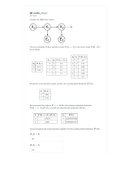
Consider the HMM shown below.
The prior probability , dynamics model , and sensor model
are as follows:
We perform a first dynamics update, and fill in the resulting belief distribution .
We incorporate the evidence . We fill in the evidence-weighted distribution
, ...
compsci 188 introduction to artificial intelligence
part i 20 points consider the hmm shown below the prior probability
and sensor model are as follows we perform a first
Written for
Electronic HW8
All documents for this subject (1)
Seller
Follow
ExamsConnoisseur
Reviews received
Content preview
Q1 HMMs, Part I
20 Points
Consider the HMM shown below.
The prior probability P (X0 ), dynamics model P (Xt+1 ∣ Xt ), and sensor model P (Et ∣ Xt )
are as follows:
We perform a first dynamics update, and fill in the resulting belief distribution B ′ (X1 ).
We incorporate the evidence E1 = c. We fill in the evidence-weighted distribution
P (E1 = c ∣ X1 )B ′ (X1 ), and the (normalized) belief distribution B(X1 ).
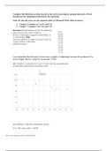
You get to perform the second dynamics update. Fill in the resulting belief distribution B ′ (X2 ).
B ′ (X2 = 0)
.80
B ′ (X2 = 1)
.20
, Now incorporate the evidence E2 = c.
Fill in the evidence-weighted distribution P (E2 = c ∣ X2 )B ′ (X2 ), and the (normalized) belief
distribution B(X2 ).
P (E2 = c ∣ X2 )B ′ (X2 ) when X2 = 0
.04
P (E2 = c ∣ X2 )B ′ (X2 ) when X2 = 1
.12
B(X2 = 0)
.25
B(X2 = 1)
.75
Q2 HMMs, Part II
20 Points
Consider the same HMM (but with different probabilities).
The prior probability P (X0 ), dynamics model P (Xt+1 ∣ Xt ), and sensor model P (Et ∣ Xt )
are as follows:
In this question we'll assume the sensor is broken and we get no more evidence readings after
E2 . We are forced to rely on dynamics updates only going forward. In the limit as t → ∞, our
~
belief about Xt should converge to a stationary distribution B (X∞ ) defined as follows:
~
B (X∞ ) := lim P (Xt ∣ E1 , E2 )
t→∞
The benefits of buying summaries with Stuvia:
Guaranteed quality through customer reviews
Stuvia customers have reviewed more than 700,000 summaries. This how you know that you are buying the best documents.
Quick and easy check-out
You can quickly pay through credit card or Stuvia-credit for the summaries. There is no membership needed.
Focus on what matters
Your fellow students write the study notes themselves, which is why the documents are always reliable and up-to-date. This ensures you quickly get to the core!
Frequently asked questions
What do I get when I buy this document?
You get a PDF, available immediately after your purchase. The purchased document is accessible anytime, anywhere and indefinitely through your profile.
Satisfaction guarantee: how does it work?
Our satisfaction guarantee ensures that you always find a study document that suits you well. You fill out a form, and our customer service team takes care of the rest.
Who am I buying these notes from?
Stuvia is a marketplace, so you are not buying this document from us, but from seller ExamsConnoisseur. Stuvia facilitates payment to the seller.
Will I be stuck with a subscription?
No, you only buy these notes for $9.99. You're not tied to anything after your purchase.