International Competitive Analysis and Strategy (EBC4044)
Summary
International Competitive Analysis and Strategy FULL Summary | | Summary Book |
18 views 1 purchase
Course
International Competitive Analysis and Strategy (EBC4044)
Institution
Maastricht University (UM)
Book
Economics of Strategy
International Competitive Analysis and Strategy FULL Summary | |
Summary of Chapter 1,2,3,4,5,6,7,8,9,10 & 12. Everything exam relevant for the exam 2022/2023. Notes, exercises from the course manual, term sheet with all relevant concepts.
Notes and explanation of figures in the book | International Competitive Analysis and Strategy | EBC4044 |
Exercises International Competitive Analysis and Strategy | Course Manual 2021-2022 |
All for this textbook (7)
Written for
Maastricht University (UM)
International Business
International Competitive Analysis and Strategy (EBC4044)
All documents for this subject (6)
Seller
Follow
lstokroos
Content preview
ICAS LFGGGGGGG
Economics Primer
1. COSTS:
1. Cost Func ons
Total Cost Function:
-total cost (TC) that the firm would incur for a level of output Q
-efficiency relationship showing the lowest possible total cost the firm
would incur to produce a level of output, given the firm’s current
technological capabilities.
-must slope upward, if firm is producing as efficiently as possible
Fixed costs (general and administrative expenses and property taxes)
remain constant as output increases (invariant to output)
Variable costs (direct labor and commissions to salespeople) increase as output increases.
Note:
- some costs (maintenance or advertising and promotional expenses) may have both fixed and variable
components
- if costs are fixed or variable depends on the time period in which decisions regarding output are contemplated
Semi-fixed costs: fixed over certain ranges of output but variable over other ranges
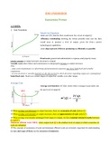
Average Cost
Average cost function (AC (Q)): shows firm’s average (or per-unit) cost
for any level of output Q
MES
TC(Q)
AC(Q) =
Q
! When average cost decreases as output increases, there are economies of scale (before Q’)
! When average cost increases as output increases, there are diseconomies of scale (after Q”)
! When average cost remains unchanged with respect to output, we have constant returns to scale (between
Q’ and Q’’)
Minimum efficient scale (MES): where output level Q′ is the smallest level of output at which economies of
scale are exhausted
! The concepts of economies of scale and minimum efficient scale are extremely important for understanding
the size and scope of firms and the structure of industries.
 ti
, Marginal Cost & Total cost
Marginal cost refers to the rate of change of total cost with respect to output.
! incremental cost of producing exactly one more unit of output.
At low levels of output (Q’) increasing
output by one unit does not change total
costs much as reflected by the low MC.
At higher levels of output (Q’’), a one-unit
increase in output has a greater impact on
total costs, corresponding MC is higher.
TC (Q + ∆ Q) − TC(Q)
MC(Q) =
∆Q
Marginal Cost & Average cost
! When average cost is decreasing (e.g., at output Q′), AC > MC,
Economies of Scale
(i.e., the average cost curve lies above the marginal cost curve).
! When average cost is increasing (e.g., at output Q′′), AC < MC,
Diseconomies of Scale
(i.e., the average cost curve lies below the marginal cost curve).
When average cost is at a minimum, AC = MC (two curves must intersect) ! Maximize profit
Short and long run average cost functions
*Long-run average cost functions: bold line
! Lowest attainable average cost for any output, when the firm
is free to adjust its plant size optimally.

,At certain levels of output, a different size of production facilities would be most efficient to realize economies
of scale and optimize average costs. If the firm knows how much output it plans to produce before building a
plant, then to minimize its costs, it should choose the plant size that results in the lowest short-run average
cost (SAC) for that desired output level.
! For output Q1, the optimal plant is a small one (lowest SAC); for output Q2, the optimal plant is a medium
one; for output Q3 and Q4, the optimal plant is a large one.
! When the firm produces Q1 in the large plant, it may need to utilize more labor to assure steady materials
flows within the large facility.
It is often useful to express short-run average costs (SAC) as the sum of average fixed costs (AFC) and
average variable costs (AVC): SAC(Q) = AFC(Q) + AVC(Q)
When volume of output increase, average fixed costs decline (cost spread over an ever-larger production
volume) while average variable costs rise. The net effect of these offsetting forces creates the U-shaped SAC
curves.
Sunk vs Avoidable costs
Sunk costs: costs that must be incurred no matter what the decision is. Cannot be avoided & not the same as
fixed costs (some fixed costs are not sunk costs)
Avoidable costs: costs that can be avoided if certain choices are made.
! The decision maker should ignore sunk costs and consider only avoidable costs.
2. ECONOMICS COSTS AND PROFITABILITY
Economic costs vs Accounting costs:
Accounting costs: Accrual accounting emphasize historical costs. Not necessarily appropriate for decision
making inside a firm. However, it is useful to compare one firm in an industry to another, or to evaluate the
financial strength of a firm, through the the accounting statements and accounting ratio analysis.
Economic costs which are based on the concept of opportunity cost (value of the best foregone alternative use
of those resources) is more appropriate for business decisions such as “when the firm must choose among
competing alternatives”. ! The economic cost of the firm’s production activities reflects a foregone opportunity
Economic profit vs Accounting profit:
Accounting Profit = Sales Revenue − Accounting Cost ! it is the net income and it excludes explicit cost
Economic Profit = Sales Revenue − Economic Cost ! it includes opportunity cost, explicit and implicit cost
= Accounting Profit − (Economic Cost − Accounting Cost)
, Accounting Profit: Simple difference between revenues Economic Profit: A concept that represents the
and expenses. difference between the accounting profits from a given
activity and the accounting profits that could have been
3. DEMAND earned by investing the same resources in the most
lucrative alternative activity.
Demand curve: quantity of a product that consumers will purchase at different
prices
! Law of demand: curve is downward sloping = the lower the price, the greater the
quantity demanded; the higher the price, the lower the quantity demanded
Price Elasticity of Demand
The price elasticity of demand (ᶯ ) is the % change in quantity
demanded brought about by a 1% change in price.
Where ΔP = P1 − P0 is the change in price, and
ΔQ = Q1 − Q0 is the resulting change
in quantity.
If ᶯ < 1 ! demand is inelastic (DA) – not price sensitive ! when price
increases, increase in sales revenues (due to only small drop in sales & charging higher price)
If ᶯ > 1! demand is elastic (DB) - price sensitive ! when price increases, decrease in sales revenues (due to
large drop in sales)
Example:
1. Suppose price is initially $5, and the corresponding quantity demanded is 1,000 units. If the price rises
to $5.75, the quantity demanded would fall to 800 units.
Q0 = 1000, Q1 = 800
P0 = 5, P1 = 5.75
! Thus over the range of prices between $5.00 and $5.75,
quantity demanded falls at a rate of 1.33% for every 1% increase in price. ᶯ > 1, therefore demand is
elastic (price senstitive), resulting in a decrease in sales revenues.
2. Suppose management believed η = 0.75. If it contemplated a 3 percent increase in price,
then it should expect a 3 x 0.75 = 2.25% drop in the quantity demanded as a result of the price increase
The benefits of buying summaries with Stuvia:
Guaranteed quality through customer reviews
Stuvia customers have reviewed more than 700,000 summaries. This how you know that you are buying the best documents.
Quick and easy check-out
You can quickly pay through credit card or Stuvia-credit for the summaries. There is no membership needed.
Focus on what matters
Your fellow students write the study notes themselves, which is why the documents are always reliable and up-to-date. This ensures you quickly get to the core!
Frequently asked questions
What do I get when I buy this document?
You get a PDF, available immediately after your purchase. The purchased document is accessible anytime, anywhere and indefinitely through your profile.
Satisfaction guarantee: how does it work?
Our satisfaction guarantee ensures that you always find a study document that suits you well. You fill out a form, and our customer service team takes care of the rest.
Who am I buying these notes from?
Stuvia is a marketplace, so you are not buying this document from us, but from seller lstokroos. Stuvia facilitates payment to the seller.
Will I be stuck with a subscription?
No, you only buy these notes for $22.75. You're not tied to anything after your purchase.