Complete summary of Empirical Methods in Finance, MSc Finance. It includes all lectures, uploaded videos and take-aways of do-files & discussion sections.
EMF part 2
Lecture 1
Volatility models & forecasting is not in the exam, but it will be in the group assignment.
Look at question 3 and question 4 on the forum and question 15.
^β is consistent (beta hat will go to beta as the sample size increases), and unbiased (Estimation of β^
is β). Beta hat is more efficient than β~ (variance of beta hat is smaller than variance of β~)
𝑉1 and 𝑉2 are consistent.
𝑉2 is unbiased but 𝑉1 has a bias.
𝑉1 is more efficient than 𝑉2.
V1 is not the BLUE (Best Linear Unbiased Estimation (BLUE)) estimator for variance. BLUE means that
of all linear unbiased estimators, this one is the best. The u in BLUE means unbiased, so V2 is not
BLUE. V2 is the unbiased one, so it will be BLUE. V1 is the most efficient consistent estimator.
The most efficient estimator is a number. One number has no variance. So we need to constrain
efficiency, because just efficiency will always be a number.
Law of iterated expectations:
For CAPM to calculate expected return, you use this law. E(R A|RM) = rf + β (Erm – rf). You take an
expectation of the total market, to calculate the expected return on asset A. It’s also called the law of
total expectation.
Some definitions (to see if the coin is fair)
Quantity of interest: fairness of the coin. So it’s something that you care about.
Parameter of interest: probability of heads (where to look to find if it’s fair). It’s a parameter
that tells you the fairness of the coin. You can also look at expected return, if you decided
that you lose $1 if it’s heads and win $1 if it’s tails.
How can you estimate the parameter of interest (probability of heads)? You need an estimate (NOT
AN ESTIMATOR). It’s a function of the data that tells you the parameter of interest. For example, the
proportion of heads (=0.45). It depends on the sample. Estimator is a function of the data (e.g. OLS),
an estimate is the number. The estimator is the proportion of heads.
We know that the proportion of heads (p^) if the sample sizen (N) is big enough. The distribution of
an estimator is normal distribution. The variance of an estimate is always zero (Because it’s a
number!). The variance of the estimator (under null hypothesis that the coin is fair) = normal
distribution.
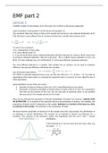
If the estimate (p~) is too far away from the mean, then you
can reject.
1
,Say that you estimate the following equation Grade = α + β (hours of study) + εi.
The estimate for β is 0.1 and the t-stat is 1.75. Is it significantly different from 0 at the 5% level. If we
use a two-sided test, it is not. However, why would we be studying more decrease in the grade? We
need to use a one-sided test, so it is statistically significant (t-stat >1.64).
A computer works in binary basis (a row of zeros and ones). The computer only reads and stores
number. so, to be able to write or read, the computer assigns to each letter a number (ASCII code).
The computer will link a number (74) to a letter (J). The computer needs to know if it needs to write a
J or 74. So, you need to tell the computer if a letter (string) or a number is coming.
So, if STATA says: ‘not possible with numeric variable’ or ‘not possible with string variable’, there’s a
type mismatch.
The computer understands five types of data
• Integers (whole numbers)
• Floats (=decimals)
• Simple (few decimals) this is the default.
• Double (many decimals; you do not need to use them)
• Strings (=text)
• Logical (=true/false; you do not need to use them)
Command: Gen int … Then you generate a variable that’s integer
We create our own type of data, if we need one for example dates. It’s counting the number of
days from the 1st of January 1960 (you can also have negative data). If you add one to the data, you
get the next day.
Example: Three trading dates and closing prices:
19/08/2022 171.52
22/08/2022 167.57
23/08/2022 167.23
Pt −Pt −1
You want to calculate returns = . But you want to look on 22/8 not to 21/8 but to 19/8
Pt −1
2022 (because of the weekends). Solution create your own calendar (that is, with trading days).
We’ll do this in the online lecture.
Then, you can also want to provide your address. You will provide, country, province, city, street
name, number. A province is within a country, city in the province, etc.. There will be no same
streetname within the city, but it will be within the country.
To find the path, you will find it by doubleclick in the area here in ‘Mijn bestanden’ and copy it:
The link between a parent folder and a child folder is represented by \ or / depending on the OS.
Key variables are variable that (combined) cannot be repeated for two observations. For example,
the combination of date and FirmName are the key variables.
2
,We can only merge two datasets if: both have the same key variable. Or the key variables of the one
data set are in the other dataset. Note that if the key variables are not the same one observation
corresponds to many observations in the other file.
In STATA, you get the error: "variable does not uniquely identify observations in the masterdata"
If both datasets contain a combination of key variables, then you cannot merge them.
YOU CANNOT FORCE STATA VIA ‘MM’ TO MERGE, AS IT WILL NOT WORK
You can merge it via sequential merging. You’re going to have a dataset with firm returns and
industry returns. You can merge a ‘dataset with firm and industry’, with a ‘dataset with monthly
returns of firms’. In that merged dataset, you can merge it again with a ‘dataset with monthly returns
of the industry’.
Stata allows us to store local (temporal) variables and files. These are variables and files that
disappear as soon as the code stops (even if it stops because of an error).
Always run the code in STATA using without selecting any lines
So after running the do-file, the local variables are gone. You cannot copy and paste to the console, it
will not work. Always run from the beginning of the code, the entire file.
Do not use temporary files until you get familiar with Stata
When using local variables, add to your code in several places: disp `var’
– Where var is the name of your variable
– This way you will be able to see the variables and make sure it is the correct value
Pre-lecture videos lecture 2
An event study refers to the econometric method to analyze the effect of a particular event on the
price of an asset. First, we need to make hypothesis. For example, the impact of some
announcement on the stock price. Say that after the announcement the stock price rose. How can we
determine that this was due to the announcement? We can compare the change in stock price with
the market. First they are quite consistent, after announcement the returns deviate. The event is
anything that might affect asset prices at a specific point in time. So we need to find the specific
point. Let define Rj,t = the return on date t of firm j if the firm j is subject to the the event. R̃ j,t the
return on date t of firm j if firm is not subject to the event. The effect of the event is the difference
between both = δj,t . The problem is we do not observe both, we cannot observe a firm that both had
and did not have the event. So we should compare a firm that’s subject to the event (E) and a firm
that is not subject to the event (NE):
But this is not a good comparison. Those firms are different.
So we should for the same firm that has the event estimate the data if they would not have the
event. We want to estimate E(δj,t | announcement). This is average treatment effect on the treated
(ATT). So we only use firms that have the event (announcement).
Say we have 3 firms, C = car manufacturer, F = film producer, T = wheel manufacturer. T = target for
acquire. If the firm buys firm T, C’s equity value would increase by 10%, F’s equity value would
decrease by 10%. ATE = average treatment effect = 10%-10%/2=0
ATT = 10%, we’ll only observe firm’s C acquiring, so ATT = 10%.
When’s ATT useful?
3
, - Evaluating a policy to foster acquisition you do not have those firms in the sample that do
not acquire
- It should be a random assigning. For example, the effect of CEO dismissal is not random. The
effect of CEO death would be a good way to use ATE. You do not want selection bias.
So, we’ll use
So the expected effect of the announcement, given that there’s been an announcement.
Rj,t is observable. E(R̃j,t | announcement) is the main object of study in Finance. You can calculate it
for example via CAPM.
So we need to do the following
1. Identify the timing of the event = define the conditioning set. |announcement
2. Model the normal return = estimate (E(R j,t | announcement)
3. Construct hypothesis: what does E(δj,t |announcement)=0 mean?
First, we’ll look at ‘|announcement’. We need to define as 0 the date of the event, usually the
announcement (of policy, information, etc.).
Then, we define an estimation period, with the following requirement. It’s the returns in this period
are not yet affected by the announcement. The period is close to the event. The period is long
enough to make the necessary estimation. It’s described by the period from T to T .
Then, we define the event period. This period might be made of one day (the event day). It usually
include all the days in which we hyopthezize an effect might exist. It’s the period from 0 to L.
So we have firms, indexed by j, with and without announcements.
Dates were indexed by t, we have every date for every firm and just once.
Now we need to transform the dataset to event time. Events are indexed by i. A firm might have
several events. If a firm has no events, it drops from the sample. Dates are in event time, indexed by
τ. Some dates might be repeated, some might drop. The market and risk-free rated for a given event-
date change over events.
Now, we’ll look at E(R̃j,t | announcement). There are four models to estimate it (i=event):
assumes that Expected return will be constant.
assumes that E(R) moves like the market
generalized way of CAPM
Fama French you extend market model by other
factors.
Model 1. We just state the mean return within the estimation window: The
advantage is that we do not need data on the market return. Hence, it is valid if the market return is
affected by the event. The disadvantage is that the estimated effect of pro-cyclical events might be
upward biased (and the other way around).
Note: T= T – T + 1
Model 2. We include the market. The advantage is there’s no estimator. On average, this model is
right. So the beta is one. Disadvantage: if firms’ exposure to market risk is related to the
announcement, the estimated effect will be biased. An example is imposing corporate taxes, this
effects Vu differently than VL .
4
The benefits of buying summaries with Stuvia:
Guaranteed quality through customer reviews
Stuvia customers have reviewed more than 700,000 summaries. This how you know that you are buying the best documents.
Quick and easy check-out
You can quickly pay through credit card or Stuvia-credit for the summaries. There is no membership needed.
Focus on what matters
Your fellow students write the study notes themselves, which is why the documents are always reliable and up-to-date. This ensures you quickly get to the core!
Frequently asked questions
What do I get when I buy this document?
You get a PDF, available immediately after your purchase. The purchased document is accessible anytime, anywhere and indefinitely through your profile.
Satisfaction guarantee: how does it work?
Our satisfaction guarantee ensures that you always find a study document that suits you well. You fill out a form, and our customer service team takes care of the rest.
Who am I buying these notes from?
Stuvia is a marketplace, so you are not buying this document from us, but from seller liekepbreure. Stuvia facilitates payment to the seller.
Will I be stuck with a subscription?
No, you only buy these notes for $9.65. You're not tied to anything after your purchase.