Summary Methods, Measurement and Statistics
Introduction to Techniques for Causal Analysis (Gelissen, 2018)
Chapter 1: Review of Basic Concepts
1.2. A simple example of a research problem
Suppose that a student wants to do a simple experiment to assess the effect of caffeine on anxiety. This simple experiment
will be used to illustrate several basic problems that arise in actual research:
1. Selection of a sample from a population.
2. Evaluating whether a sample is representative of a population.
3. Descriptive versus inferential applications of statistics.
4. Levels of measurement and types of variables.
5. Selection of a statistical analysis that is appropriate for the type of data.
6. Experimental design versus nonexperimental design.
Each of the following sections describes common practices in actual research in contrast to idealized textbook approaches.
1.4. Samples and populations
• Sample: a subset of members of a population. The researcher selects a sample from the population using either
simple random sampling or other sampling methods.
• Simple random sample: if a sample is chosen randomly from a population, it should be representative of the
population which it is drawn. A sample is representative if it has characteristics similar to those of the population.
For example, if the population has a mean age of 25 years and is 60% female and 40% male, the sample would be
representative if it is similar to the population.
• Accidental or convenience sample: sample consists of participants who are readily available to the researcher.
• Bias: a systematic difference between the characteristics of a sample and a population.
1.5. Descriptive versus inferential uses of statistics
• Descriptive statistics: statistics that are used only to describe and summarize information about a sample. Reduce
the date to understandable pieces of information.
• Inferential statistics: statistics that are used to draw inferences about populations. In practice we only have
observations on a selection of cases from a larger population. We need to evaluate whether the results in the
sample are generalizable to the population.
1.6. Levels of measurement and types of variables
The classic levels of measurement:
- Nominal data: numbers express group membership. Nominal variables classify cases into two or more categories.
Categories must be exhaustive (all possibilities should be covered) and mutually exclusive (every case fit into one
category and one category only).
o Marital status: 1 = single, 2 = married, 3 = in a serous relationship, 4 = not specified otherwise.
- Ordinal data: numbers express an ordering. Numbers expresses more or less of a quantity, but the difference
between 1 and 2 is not the same in quantity than between 2 and 3, 3 and 4, and so on.
o Smoking intensity: 1 = never, 2 = occasionally, 3 = regularly (at least 1 cigarette per day), 4 = heavy (more
than 5 cigarettes per day).
- Interval and ratio (scale level): numbers express differences in quantity using a common unit.
o The difference between 70 and 80 IQ points is comparable to a difference between 100 and 110. Both
span a difference of 10 units. Likewise, if on Monday the temperature is 30 degrees, on Tuesday 25
degrees and Wednesday, 15 degrees, then we can say that the temperature drop between Tuesday and
Wednesday is twice as large as the drop between Monday and Tuesday.
o Ratio-level data have a ‘natural’ zero-point (e.g., length, income). As a result, you can compare the relative
magnitude of things, e.g. you can say that one person is twice as tall as another person.
o Interval level variables don’t have a natural zero point (e.g., zero temperature is meaningless), but it is
arbitrarily chosen and can differ across scales.
1
,Both interval and ratio-level data are referred to as scale data. The idea is simple: all variables that are not nominal or
ordinal are treated as scale-level variables. These are also the levels that SPSS uses. Measurement level is a property of
the measurement values, it is not an intrinsic property of a variable. E.g., you cannot say that “body height” has interval
level; length can be measured at different levels (think of your gym-class). So, there is not necessarily a one-to-one
relationship between measurement levels and variables. Measurement levels determine the kind of statistics and
statistical analyses you can use meaningfully. For example, the mean of a nominal variable is meaningless (e.g., “the
average eye color). Hence, for the analyses you should always respect the measurement le vels of the variables envisaged.
Many of the commonly used statistical techniques assume scale data. However, for many variables in the social sciences,
it is not evident that data are interval level (e.g., political interest) Therefore, it is common practice to simply assume that
we have acquired interval data, without worrying too much if this is true and this turns out to be very useful.
Two types of variables:
1. Categorical variable: may represent naturally occurring groups or categories (nominal data, 1 = female, 2 = male).
2. Quantitative variable: have scores that provide information about the magnitude of differences between
participants in terms of the amount of some characteristic (ordinal, interval, ratio, 1 = most anxious, 2 = second
most anxious, think of Likert scales, scale from 1 to 5).
Every analysis starts with data inspection, its goal is to get a clear picture of the data by examining one variable at the time
(univariate), or pairs of variables (bivariate). To accomplish this goal, we use graphs and statistics. Which statistics and
graphs are most appropriate depends on the measurement level (i.e., whether the data are nominal, ordinal, or scale
level). In general, we want to know more about:
- Central tendency: What are the most common values? (Mean, Modus, Median)
- Variability: How large are the differences between the subjects? Are there extreme values in the sample?
- Bivariate Association: for each pair of variables, do they associate/covary (i.e., do low/large values on one variable
go together with low/large values on the other variable.
1.7. The normal distribution
Bar charts (nominal and ordinal data) Histogram (scale data)
Central tendency
- Mode: the score that is observed most frequently
- Median: the score that separates the higher half of data from the lower half
o Example 1: (N = unequal): 4, 5, 6, 7, 8, 9, 9 = median is 7
o Example 2: (N = equal): 4, 5, 6, 8, 9, 9 = median is 7 (mean of the two middle values 6 and 8).
𝛴𝑋 𝑠𝑢𝑚 𝑜𝑓 𝑎𝑙𝑙 𝑠𝑐𝑜𝑟𝑒𝑠
- Mean: 𝑀 = =
𝑁 𝑡𝑜𝑡𝑎𝑙 𝑛𝑢𝑚𝑏𝑒𝑟 𝑜𝑓 𝑠𝑐𝑜𝑟𝑒𝑠
Minimum, maximum, range, and interquartile range
- Minimum = lowest observed value; maximum = highest observed value.
- Range = maximum – minimum
- IQR = ranges of scores that encompass 50% of the middle observations; thus, excluding the 25% lowest and 25%
highest observations.
2
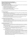
, A theoretical distribution shape
that is of particular interest in
statistics is the normal distribution
illustrated in the figure. The curve
is symmetrical, with a peak in the
middle and tails that fall of
gradually on both sides. The
normal curve is often described as
a bell-shaped curve.
µ is the mean that is the center of
the distribution. µ is estimated by
a sample mean M.
σ is the standard deviation that is,
it corresponds to the dispersion of
the distribution. σ is estimated by
the sample standard deviation,
usually denoted by either s or SD.
Normal distribution with μ = 0 and standard deviation σ = 1. Notice that if 𝑋 is not normally distributed then 𝑍 scores are
not normally distributed as well.
Chapter 2: Basic statistics, sampling error and confidence intervals
2.1. Introduction
In scientific social-research we seek knowledge that is generally true for a whole class of units. The whole class is the
population. We observe some objects in a sample: a selection of subjects from the population. We want to extend our
findings in the sample to the whole population. We take sample values as our ‘best guess’ for the unknown population
value. In other words, the sample value is an estimate of the population value. To correctly use statistics, it’s important to
precisely distinguish between (unknown) population values (denoted by Greek letters) and the observed sample values
both in the language as in the symbols. Characteristics of populations (mean, proportions) → parameters. Sample
estimates of the population characteristics → statistics.
Name of statistic Sample statistic Population parameter Pronunciation Greek letter
Mean M (or ̅ X) 𝑥̅ µ Mu
Standard deviation s or SD (or ŝ) σ Sigma
Variance s2 (or ŝ 2) σ2 Sigma squared
Distance of individual X (X−M) ̅)
(X−X (X − µ) -
z= or z = z=
score from the mean s SD
σ
Standard error of the SEM (or SEx ̅) σM (or σx ̅) -
sample mean
Sample results will vary from sample to sample. Each time we draw a new sample, the composition of the sample is
different, and the results will be slightly different. This variability across samples are sampling fluctuations. As another
consequence, sample values will not exactly be equal to the population value, that is, the sample value will most often be
close to, but not exactly equal the population value. Differences between sample values and population values are known
as sampling errors. It is the error we make if we use the sample value as our best guess of the population value. We use
inferential statistics to take sampling errors into account when drawing conclusions about populations from sample
results.
2.3. Sample Mean (M)
A sample mean provides information about the size of a ‘typical’ score in a sample. We use sample means to draw
conclusions about population means. However, each random sample has a different composition. By chance you may
3
The benefits of buying summaries with Stuvia:
Guaranteed quality through customer reviews
Stuvia customers have reviewed more than 700,000 summaries. This how you know that you are buying the best documents.
Quick and easy check-out
You can quickly pay through credit card or Stuvia-credit for the summaries. There is no membership needed.
Focus on what matters
Your fellow students write the study notes themselves, which is why the documents are always reliable and up-to-date. This ensures you quickly get to the core!
Frequently asked questions
What do I get when I buy this document?
You get a PDF, available immediately after your purchase. The purchased document is accessible anytime, anywhere and indefinitely through your profile.
Satisfaction guarantee: how does it work?
Our satisfaction guarantee ensures that you always find a study document that suits you well. You fill out a form, and our customer service team takes care of the rest.
Who am I buying these notes from?
Stuvia is a marketplace, so you are not buying this document from us, but from seller annevandentillaar. Stuvia facilitates payment to the seller.
Will I be stuck with a subscription?
No, you only buy these notes for $7.46. You're not tied to anything after your purchase.