Summary Management Research Methods 2 (MRM BA2): Received grade: 8.0 ()
48 views 4 purchases
Course
Management Research Methods 2 (6012S0049Y)
Institution
Universiteit Van Amsterdam (UvA)
I made a summary of Management Research Methods 2 which contains additional lecture notes and really helpful notes from the homework I had to do. This elaborate summary will help you with your upcoming exam, as my grade was an 8.0. If you also do the exercises given in class, you should be fine! T...
In research: by “model” we mean a simplified description of reality.
In social sciences we often treat ordinal scales as (pseudo) interval scales, e.g. Likert scales.
ANOVA: Analysis Of Variance. Test whether different groups score differently on a quantitative
outcome.
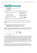
Two measurements of variability (how much values differ in your data) are:
- Variance: average of the squared differences from the mean.
- Sum of Squares: sum of the squared differences from the mean.
MRM2 students are assigned to three subgroups, each group receives a different teaching method.
One thing could be to check if there are difference in scores on the exam between the groups.
Which group scores best overall and which scores worst? How can we investigate with a certain level
of (statistical) confidence, what differences there might be between the groups? → ANOVA. This
does help by comparing the variability between the groups against the variability within the groups.
In other words, does it matter in which group you are (which teaching method you receive) with
regard to your exam score? We want to see much of the variability (differences) in our outcome
variable can be explained by our predictor variable. However, we probably won’t be able to explain
all the differences (all the variability) in exam scores, solely by creating our groups who receive
different teaching methods.
VB: If scores on a quantitative outcome vary more WITHIN groups than BETWEEN groups, for
example exam scores for three groups of students who each received a different teaching method.
It then is unlikely that it matters which group you are in, regarding your score on the outcome.
1
,ANOVA statistically examines how much of the variability in our outcome variable can be
explained by our predictor variable. It breaks down variability through calculating sums of squares.
Via these calculations, the ANOVA helps us test if the mean scores of the groups are statistically
different from each other.
Assumptions one way between-subjects ANOVA:
- Predictor Variable (PV) = Categorical with more than 2 groups
- Outcome Variable (OV) = Quantitative
Variance is homogenous across groups → Levene’s test
Groups are roughly equally sized → in this class they always are.
Our subjects can only be in one group (between subjects design).
Residuals are normally distributed → in this class we don’t test for this.
NOT adhering to assumptions can produce invalid outcomes!
Example
Question: Is there a relation between shopping platform
and customer satisfaction?
PV = shopping platform. Categorical, with three levels:
1. Brick-and-mortar store
2. Web shop
3. Reseller
This one PV, more accurately, an equation containing this one PV, is our statistical model in this analysis.
OV = customer satisfaction. Quantitative
- Scores from 1-50
We have 10 observations on customer satisfaction scores (OV).
The grand overall mean (denoted by ydakje) is equal to 32.3
2
,SS (Sum of Squares): quantification of variability of scores of a quantitative outcome.
SStotal: The total variability in scores on an outcome variable, on an outcome variable.
We have now decomposed the variability in our data in a part that can be explained by:
➢ Our model = between group SS (high as possible)
➢ A residual part = within group SS (error, low as possible, similar groups)
We can now calculate the proportion of the total variance in our data that is “explained” by our
model. This ratio to calculate this is called R2. The higher the R2, the better; it can better explain the
variability.
we can explain 95,7% of
the differences in scores
on or OV, by our model.
3
, To investigate if the group means differ with an ANOVA, we do a F-test. This is a statistical test and
thus checks the ratio explained variability to unexplained variability. High value is better.
F-test
H0: all the mean scores of groups on the outcome variable are the same.
HA: at least one of the mean scores of the groups on the outcome variable differs from the others.
VB: Obtaining an F value of 11 tells us that we have 11 times more explained variance than
unexplained variance in our dataset.
However, we cannot just divide the model sum of squares by the residual sum of squares, because
they are not based on the same number of observations and thus not have an ‘equal weight’. We
therefore divide by the degrees of freedom and get something called the “mean square” (average
sum of squares).
!! As with any test statistic, the F-ratio has a null hypothesis and an alternative hypothesis:
As with any test statistic (in this case ”F”) it has an accompanying p value, which tells us: the
probability of obtaining a result (or test-statistic value) equal to (or ‘more extreme’) than what was
observed (the result you got), assuming that the null hypothesis is true. Based on the p value you can
either reject or not reject the null hypothesis. The p value stands for the probability of obtaining the
observed test statistic, or one more extreme, under assumption null hypothesis is true.
If we have three groups in our single PV (One way ANOVA), each group will have mean (average)
score on the OV, and a variance (measure for how much the scores differ within the groups).
We can test whether the means between
the groups statistically differ → F test.
We can also test whether the variances
between the groups statistically differ →
Levene’s test.
1. Check descriptive statistics
2. Check Levene is > 0,05 (variances are equal)
3. Check ANOVA output. <0,05 means there is a significant difference between groups.
4
The benefits of buying summaries with Stuvia:
Guaranteed quality through customer reviews
Stuvia customers have reviewed more than 700,000 summaries. This how you know that you are buying the best documents.
Quick and easy check-out
You can quickly pay through credit card or Stuvia-credit for the summaries. There is no membership needed.
Focus on what matters
Your fellow students write the study notes themselves, which is why the documents are always reliable and up-to-date. This ensures you quickly get to the core!
Frequently asked questions
What do I get when I buy this document?
You get a PDF, available immediately after your purchase. The purchased document is accessible anytime, anywhere and indefinitely through your profile.
Satisfaction guarantee: how does it work?
Our satisfaction guarantee ensures that you always find a study document that suits you well. You fill out a form, and our customer service team takes care of the rest.
Who am I buying these notes from?
Stuvia is a marketplace, so you are not buying this document from us, but from seller romytempelman. Stuvia facilitates payment to the seller.
Will I be stuck with a subscription?
No, you only buy these notes for $9.19. You're not tied to anything after your purchase.