Summary of the required articles/parts of books for the course Data Science Methods for MADS of the University of Groningen. At some points summaries of the reading list are extended with information from the lecture to make explanations more clear.
The included articles/parts of books are:
- ...
Analyzing larger sets of data may require significant computational power, which can be handled by sub-sampling. Instead
of analyzing the whole sample, observations from the large data sample can be randomly drawn to be analyzed as a
representative sample of the original sample. However, this is less favorable in a big data setting, since the amount of
noise within the data also increases when data from various data sources is combined.
§ Data from different sources may partially be miss-aligned;
§ There may be coding issues;
§ Faulty data collection mechanisms, or
§ Non-representative sources may negatively affect the quality of some observations and may leave others unaffected.
In case of sub-sampling the amount of noise may lead to critical biases, which may endanger the reliability and validity of
findings and prevent generalizing from the subsample to the whole data set (“n equals all” paradox). Noise may cause
harm in case of smaller (sub) samples, but is usually outperformed in presence of very large data sets that contain all sort
of observations available to a researcher. Due to these performance issues, marketing research is using estimation
techniques and modeling approaches referred to as Machine Learning algorithms.
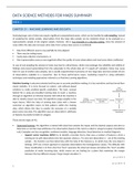
Machine learning is outcome-oriented and focuses on accurate prediction making. It is less restrictive and less formal than
classic statistics. It is more focused on system- and software-based
solutions to make problem-specific predictions. The basic concept
behind ML is using pre-classified training data to teach a machine
through an algorithm an inferred function with which the machine is
able to classify unseen new data. ML algorithms assign weights to the
input factors. With the help of training data (data with a known
outcome) an algorithm learns to find patterns within the training
data, which allows him later to predict the outcome of a variable
given some new data. The algorithm uses an observation’s attributes
or features to predict its label or category.
There are two types of ML:
§ Supervised learning: the algorithm is trained with data that contains the inputs and the desired outputs and aims to
determine a rule that maps attributes of an observation (inputs of the rule) to a label or category (output of prediction
rule). Examples are face recognition, sentiment analysis, language detection, fraud detection or medical diagnosis.
o Support vector machines (SVM) try to identify a function f(xi)=yi that uses a number of features x i from a
training set to split observations into two separate classes y i. For any new observation n – out of the training
sample – the function can then determine with the help of the features x n to which class the new object n
belongs. SVM use a linear approach to separate observations into homogeneous classes. The difficulty with
linear classification is to find a line that “best” separates the observed classes and allows the “best” possible
prediction of newly incoming data, which means we are looking for a plane that maximizes the margin
between the two different classes (“large margin classifiers”).
1
, In case of a linear separation problem with two classes, it can be
formally defined as depicted on the right. The formulas express the two
borders on the edges of the hyperplane that separates the two classes 1
and -1 (support vectors). ω represents a normalized vector to the
hyperplane and the offset of the vector from the origin. ω and b can be
combined to express the distance between the two support vectors
2
which is . To find the hyperplane that maximizes the distance
¿|ω|∨¿ ¿
2
between the two support vectors ||ω || needs to be minimized.
¿|ω|∨¿ ¿
Since no observation of the training data must fall into the
margin of the hyperplane, a reformulation is needed:
This leads to the following optimization problem:
Commonly this is achieved with the help of a simple Lagrange approach where one tries to maximize the
Lagrange operator α while minimizing b and ω . A SVM algorithm starts with estimating the Lagrange
operator α I for the two support vectors. Then the algorithm uses the information from the two support
N
vectors to determine the separating “middle” vector ω of the hyperplane with ω = ∑ α y x . This approach
i i i
i=1
only works with linearly separable data. For data that cannot be
linearly split into groups, one may relax the rules for the margin and
allow few “misclassified” observations to be within the margin (soft
margin machines). This can be reformulated to:
Here C is a constant that balances the width of the margin and the amount of misclassification of data points
and ξ I represents the misclassification of observation i. this approach is still based on a linear separation
function.
In cases where problems are not separable with a linear approach, data may be
split up in a more dimensional space to find a plane that helps to separate the
data into groups (Kernel based support vector machines). Here φ (x) depicts a function that is mapping the
data into another space. The kernel function applies some transformation to the feature vectors x i and xj and
combines the features using a dot product, which takes the vectors of the two input features and returns a
single number. Doing so, one can apply different forms of transformation. Kernel functions take different
forms with the most basic one using a linear combination that simply forms the dot products of the different
input features:
Polynomial Kernels of degree d use a simple non-linear transformation of the data:
Non-linear Kernels usually require more testing efforts and commonly result in longer training times. Such
Kernel extensions are therefore frequently used for more complex classification tasks such as image or face
recognition.
o Decision tree models start out with the complete training set and determine a series of splits to create more
homogenous sub-groups with the goal of creating a classification that is as good as possible, with a minimum
number of splits. At each split, a variable is selected that forms the basis for a decision rule that drives the
2
, split. In most cases, a “greedy” strategy is followed, where the variable and the thresholds for the associated
decision rule are selected that result in the greatest improvement in the classification. At each step in the
creation of a decision tree, it is determined whether additional splits will lead to better classifications.
A tree by default accommodates interaction effects and nonlinearities. A tree can account for
nonlinearities by splitting on the same variable twice. Having suitable training data with enough
attributes one can develop larger models with more nodes and leaves accounting for many
interactions between the different available variables.
Tree-structured models are popular in practice, as they are easy to follow and to understand. As
they are robust to many data problems and rather efficient in determining classes, they are included
in many status-quo data mining packages.
Decision tree learning models can also be applied to continuous outcome variables. In these cases
two other measures for impurity are commonly used: Gini Impurity and Variance Reduction. Both
measure impurity within the resulting groups of a split, but variance reduction is mostly used with
continuous variables. Variance reduction consists of comparing how much the variance within a leaf
is decreased given a split variable compared to other split variables.
Tree models using classical impurity measures are commonly referred to as Classification and
Regression Trees (CART) models. Tree models using chi-square tests are referred to as Chi-squared
Automatic Interaction Detector (CHAID) models, which rely on a three-step process to build up a
tree:
1. Merging: the algorithm cycles through all predictors testing for significant differences
between outcome categories with respect to the dependent variable. If the difference for a
given pair of predictor categories is not statistically significant (according to a threshold
determined by the research called alpha-to-merge value) the algorithm merges the
predictor categories and repeats this step.
2. Splitting: For all pairings with a significant difference, the algorithm will continue to
calculate a p-value (based on a Bonferroni adjustment). It then continues to find the pairing
with the highest similarity, which is indicated by the lowest statistical difference, i.e. the
highest p-value. This pairing is then used to split the leaf.
3. Stopping: The algorithm stops growing the tree in case that the smallest p-value for any
predictor is greater than a pre-set threshold commonly called alpha-to-split value.
CHAID models can deal with different types of dependent variables. They deliver powerful and
convenient alternatives to traditional CART models, however, merging and stopping decisions are
largely affected by the alpha-values the researcher has to pre-determine. An extension that
continues the merging process until only two categories remain for each predictor was therefore
introduced, which does not need an alpha-to-merge variable: exhaustive CHAID models.
Compared to CART models, CHAID models take more computational time and computational power.
Especially in the case of data sets with many (continuous) variables and many observations this may
become a serious limiting issue.
QUEST (Quick, Unbiased, Efficient, Statistical Tree) relies on Fisher’s Linear Discriminant Analysis
(LDA) for splitting leaves. QUEST uses LDA to determine the dominant predictor at each leave and
then continues growing the tree. QUEST is the most efficient in terms of computational resources
but is only able to cope with binary outcomes.
Decision trees have the problem of overfitting. Using only one tree model may lead to very specific
prediction outcomes that are unique to the training data. One way to deal with this is pruning,
which develops trees with the loosest possible stopping criterion. The resulting, overfitting tree is
then cut back by removing leaves, which are not contributing to the generalization accuracy.
3
, A very common pruning approach is reduce-error-pruning: while going from the bottom to
the top through each leaf, it checks whether replacing a leaf with the most frequent
category does not reduce the tree’s accuracy. If this is true, the leaf gets pruned.
There is no golden rule regarding pruning methods. Another way to deal with overfitting is
combining different tree models together aggregating decision rules across different tree models:
ensemble methods with most common methods:
Bagging decision trees: a number of data sets are created, consisting of random draws with
replacement from the main training set. These created data sets are usually of the same
size as the full training set, so that some observations appear more than once in any of
these data sets. Each set is then used to train a decision tree. When a new data point needs
to be classified, the N resulting trees each generate a classification for the new data point.
The results of each tree are then aggregated when assigning the final category for the new
observation. This is typically done by means of a majority vote over the N classifications.
Even though each subset tree may overfit, results show that the mean model delivers
acceptable generalizable results.
Random forest classifiers: if one or a few features are very strong predictors for an
outcome variable, correlation may occur between trees. A solution is random forests,
where the adapted algorithm selects at each feature split in the learning process, a random
subset of the features following a random subspace method.
Boosted decision trees: estimators are built sequentially; boosting works with reweighted
versions of the original training set. The algorithm starts out with the original version of the
training data set, where each observation has the same weight. The weights for the second
step are determined based on the misclassifications that result when applying a tree to the
data. The misclassified observations receive a higher weight in the next step of the boosting
algorithm, since a stronger focus on these observations increases accuracy of subsequent
steps in the algorithm. The final classification is based on a weighted vote across the
sequential classifications, where better classifications get a higher weight. It is especially
suitable in case of different types of predictor variables and in presence of missing data.
Boosting further allows outliers and does not require any form of data transformation. It
can further fit complex nonlinear relationships. Boosting regression trees tend to
outperform random forests and classic bagging trees in case of non-skewed data.
o Naïve Bayes (NB) tries to infer information from training data and to build rules that the (co)-occurrence of
certain features determines the membership in different classes. All NB classifiers rely on the basic Bayesian
Theorem:
Where p(A|B) represents the probability that we can classify an observation to class A, given that we observe
behavior B: the posterior. P(B|A) expresses the probability that the attribute B occurs, given that the
observation belongs to class A. P(A) is the general probability of occurrence of class A, and the third part
(p(B)) is the general probability of occurrence of B. Bayes Theorem can be adapted to all types of
classification problems where we observe a certain number of features for different items and where we
want to determine the probability that an item belongs to a certain class.
For every new observation of X, the classifier will predict that the observation belongs to the class that
results with the highest a posteriori probability depending on the
presence of X: X can thus only be classified as belonging to class C i if p(Ci|X) is highest among all k posterior
probabilities, which is referred to as the maximum posteriori hypothesis,
leading to: which expresses the probability of X belonging to class C i as the product
4
The benefits of buying summaries with Stuvia:
Guaranteed quality through customer reviews
Stuvia customers have reviewed more than 700,000 summaries. This how you know that you are buying the best documents.
Quick and easy check-out
You can quickly pay through credit card or Stuvia-credit for the summaries. There is no membership needed.
Focus on what matters
Your fellow students write the study notes themselves, which is why the documents are always reliable and up-to-date. This ensures you quickly get to the core!
Frequently asked questions
What do I get when I buy this document?
You get a PDF, available immediately after your purchase. The purchased document is accessible anytime, anywhere and indefinitely through your profile.
Satisfaction guarantee: how does it work?
Our satisfaction guarantee ensures that you always find a study document that suits you well. You fill out a form, and our customer service team takes care of the rest.
Who am I buying these notes from?
Stuvia is a marketplace, so you are not buying this document from us, but from seller RUGstudent123. Stuvia facilitates payment to the seller.
Will I be stuck with a subscription?
No, you only buy these notes for $7.47. You're not tied to anything after your purchase.